Showing posts with label Oracle Data Miner. Show all posts

Wednesday, December 11, 2013

Running PL/SQL Procedures in Parallel

As your data volumes increase, particularly as you evolve into the big data world, you will be start to see that your Oracle Data Mining scoring functions will start to take longer and longer.  To apply an Oracle Data Mining model to new data is a very quick process. The models are, what Oracle calls, first class objects in the database. This basically means that they run Very quickly with very little overhead.

But as the data volumes increase you will start to see that your Apply process or scoring the data will start to take longer and longer. As with all OLTP or OLAP environments as the data grows you will start to use other in-database features to help your code run quicker. One example of this is to use the Parallel Option.

You can use the Parallel Option to run your Oracle Data Mining functions in real-time and in batch processing mode. The examples given below shows you how you can do this.

Let us first start with some basics. What are the typical commands necessary to setup our schema or objects to use Parallel. The following commands are examples of what we can use

ALTER session enable parallel dml;
ALTER TABLE table_name PARALLEL (DEGREE 8);
ALTER TABLE table_name NOPARALLEL;
CREATE TABLE … PARALLEL degree …
ALTER  TABLE … PARALLEL degree …
CREATE INDEX … PARALLEL degree …
ALTER  INDEX … PARALLEL degree …

You can force parallel operations for tables that have a degree of 1 by using the force option.

ALTER SESSION ENABLE PARALLEL DDL;
ALTER SESSION ENABLE PARALLEL DML;
ALTER SESSION ENABLE PARALLEL QUERY;

alter session force parallel query PARALLEL 2

You can disable parallel processing with the following session statements.

ALTER SESSION DISABLE PARALLEL DDL;
ALTER SESSION DISABLE PARALLEL DML;
ALTER SESSION DISABLE PARALLEL QUERY;

We can also tell the database what degree of Parallelism to use


ALTER SESSION FORCE PARALLEL DDL PARALLEL 32;
ALTER SESSION FORCE PARALLEL DML PARALLEL 32;
ALTER SESSION FORCE PARALLEL QUERY PARALLEL 32;


Using your Oracle Data Mining model in real-time using Parallel


When you want to use your Oracle Data Mining model in real-time, on one record or a set of records you will be using the PREDICTION and PREDICTION_PROBABILITY function. The following example shows how a Classification model is being applied to some data in a view called MINING_DATA_APPLY_V.


column prob format 99.99999
SELECT cust_id,
       PREDICTION(DEMO_CLASS_DT_MODEL USING *)  Pred,
       PREDICTION_PROBABILITY(DEMO_CLASS_DT_MODEL USING *) Prob
FROM   mining_data_apply_v
WHERE  rownum <= 18
/


   CUST_ID       PRED      PROB
---------- ---------- ---------
    100574          0    .63415
    100577          1    .73663
    100586          0    .95219
    100593          0    .60061
    100598          0    .95219
    100599          0    .95219
    100601          1    .73663
    100603          0    .95219
    100612          1    .73663
    100619          0    .95219
    100621          1    .73663
    100626          1    .73663
    100627          0    .95219
    100628          0    .95219
    100633          1    .73663
    100640          0    .95219
    100648          1    .73663
    100650          0    .60061


If the volume of data warrants the use of the Parallel option then we can add the necessary hint to the above query as illustrated in the example below.


SELECT /*+ PARALLEL(mining_data_apply_v, 4) */
       cust_id,
       PREDICTION(DEMO_CLASS_DT_MODEL USING *)  Pred,
       PREDICTION_PROBABILITY(DEMO_CLASS_DT_MODEL USING *) Prob
FROM   mining_data_apply_v
WHERE  rownum <= 18
/


If you turn on autotrace you will see that Parallel was used. So you should now be able to use your Oracle Data Mining models to work on a Very large number of records and by adjusting the degree of parallelism you can improvements.


Using your Oracle Data Mining model in Batch mode using Parallel


When you want to perform some batch scoring of your data using your Oracle Data Mining model you will have to use the APPLY procedure that is part of the DBMS_DATA_MINING package. But the problem with using a procedure or function is that you cannot give it a hint to tell it to use the parallel option. So unless you have the tables(s) setup with parallel and/or the session to use parallel, then you cannot run your Oracle Data Mining model in Parallel using the APPLY procedure.


So how can you get the DBMA_DATA_MINING.APPLY procedure to run in parallel?


The answer is that you can use the DBMS_PARALLEL_EXECUTE package. The following steps walks you through what you need to do to use the DMBS_PARALLEL_EXECUTE package to run your Oracle Data Mining models in parallel.


The first step required is for you to put the DBMS_DATA_MINING.APPLY code into a stored procedure. The following code shows how our DEMO_CLASS_DT_MODEL can be used by the APPLY procedure and how all of this can be incorporated into a stored procedure called SCORE_DATA.


create or replace procedure score_data
is
begin


dbms_data_mining.apply(
  model_name => 'DEMO_CLAS_DT_MODEL',
  data_table_name => 'NEW_DATA_TO_SCORE',
  case_id_column_name => 'CUST_ID',
  result_table_name => 'NEW_DATA_SCORED');


end;
/


Next we need to create a Parallel Task for the DBMS_PARALLEL_EXECUTE package. In the following example this is called ODM_SCORE_DATA.


-- Create the TASK
  DBMS_PARALLEL_EXECUTE.CREATE_TASK ('ODM_SCORE_DATA');


Next we need to define the Parallel Workload Chunks details

 -- Chunk the table by ROWID
DBMS_PARALLEL_EXECUTE.CREATE_CHUNKS_BY_ROWID('ODM_SCORE_DATA', 'DMUSER', 'NEW_DATA_TO_SCORE', true, 100);
The scheduled jobs take an unassigned workload chunk, process it and will then move onto the next unassigned chunk. 
 
Now you are ready to execute the stored procedure for your Oracle Data Mining model, in parallel by 10.

DECLARE
   l_sql_stmt   varchar2(200);
BEGIN
   -- Execute the DML in parallel
   l_sql_stmt := 'begin score_data(); end;';
  
   DBMS_PARALLEL_EXECUTE.RUN_TASK('ODM_SCORE_DATA', l_sql_stmt, DBMS_SQL.NATIVE,
                                  parallel_level => 10);
END;
/


When every thing is finished you can then clean up and remove the task using


BEGIN
   dbms_parallel_execute.drop_task('ODM_SCORE_DATA');
END;
/


NOTE: The schema that will be running the above code will need to have the necessary privileges to run DBMS_SCHEDULER, for example


grant create job to dmuser;

Tuesday, December 3, 2013

Non-running workflows in ODMr 4 EA3

If you are brave enough to be using the early adopter releases of ODMr you may have run into the issue with your workflows not running.

When you go to run your workflow you will get the following window and nothing else happens.

image

To get passed this you will need to kill SQL Developer using the task manager or equivalent.

So how do you stop this from happening so that you can get your workflows to run. The simple solutions is that you need to have the workflow tab open for the workflow to run correctly.

To do this you need to make Oracle Data Miner visible, by selecting Tools from the menu, then Data Miner and finally Make Visible

image

Then you will need to go to the View menu option, then select Data Miner and then Workflow Jobs

image

Now your workflows will work and complete.

Hopefully this will be fixed in the production release of ODMr 4 (SQL Developer 4)

Wednesday, October 9, 2013

How to Fix Odd Layout Behaviour in ODM v4 EA1 & EA2

If you have been using the last versions of the Oracle Data Miner tool that have been released as part of SQL Developer 4 EA1 and EA2, you may have noticed that the layout of your worksheets and other areas are inconsistent each time you open ODM.

This can be very frustrating as you have to rearrange the layout of the worksheets, property inspection, the ODM connections tab, etc, etc, etc.

This “feature” seems to be linked to when you installed the new version of the software. When you open SQL Dev 4 EA1 & EA2 you are asked if you would like to migrate your settings.  If you selected Yes for this then it is this that is causing the project.

How do you fix this?

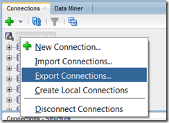
1. Export your SQL Developer Connections. To do this go to the Connections tab and right click on Connections and select export from the menu

image

This will create a XML file.  Save this to your desktop so that you can find it easily later.

2. Locate the AppData directory for SQL Developer.  This really depends on your environment. If you are using Windows for your client then the AppData directory will be located somewhere live the following

C:\Users\<your username>\AppData\Roaming\SQL Developer

3. Rename the System4.0… Directory.  Located in the AppData/SQL Developer directory called some like  ‘system4.0.0.12.84’  if you have installed and migrated to SQL Dev 4 EA2.  Rename this directory to another name e.g. ‘system4.0.0.12.84_old’.  This effectively deletes all your setting for SQL Developer 4

4. Start SQL Dev 4.  When you start SQL Developer 4 EA1 or EA2 it will be like you are running the software for the first time.  But this time, when you are asked do you want to migrate your setting from an earlier version, select No.  This will create a clean system folder.

5. Import your Connections.  When SQL Developer opens you can right click on the connection link and select Import Connections (see image above). Then enter the name and location of the file you create in step 1 above.


After completing all of the above steps your unusual layout when you open ODM should now be fixed.

Tuesday, September 24, 2013

Adding Oracle Data Miner to OBIEE

Oracle Data Miner is a very powerful tool that provides advanced machine learning algorithms that are embedded in the Oracle database. By using Oracle Data Miner you do not have to use another tool, from another vendor, to do your data mining. You can do everything in the database, ensuring that the security of your data is maintained and use all the performance functionality that comes with the database.
To add to the advanced insights that you can get from using ODM, you can combine ODM with your OBIEE dashboards to gain a deeper level of insight of your data. This is the combining of data mining techniques and visualization techniques.
The purpose of this blog post is to show you the steps involved in adding an ODM model to your OBIEE dashboards. Lots of people have been asking for the details of how to do it, so here it is.
The following example is based on a presentation that I have given a few times (OUG Ireland, UKOUG, OOW) with Antony Heljula.
1. Export & Import the ODM model
If your data mining analysis and development was completed in a different database to where your OBIEE data resides then you will need to move the ODM model from ODM/development database to the OBIEE database.
ODM provides two PL/SQL procedures to allow you to easily move your ODM model. These procedures are part of the DBMS_DATA_MINING package. To export a model you will need to use the DBMS_DATA_MINING.EXPORT_MODEL procedure. Similarly to import your (exported) ODM model you will use the DBMS_DATA_MINING.IMPORT_MODEL procedure.
2. Create a view that uses the ODM model
You can create a view that uses the PREDICTION and PREDICTION_PROBABILITY functions to apply the import ODM model to your data. For example the following view is used to score our customer data to make a prediction of they are going to churn and the probability that this prediction is correct.
SELECT st_pk,
       prediction(clas_decision_tree using *) WITHDRAW_PREDICTION,
       prediction_probability(clas_decision_tree using *) WITHDRAW_PROBABILITY
FROM   CUSTOMER_DATA;

clip_image002
3. Import the view into the Physical layer of the BI Repository (RPD)
The view was then imported into the Physical layer of the BI Repository (RPD) where it was joined on primary key to the other customer tables (we had one records per customer in the view). With the tables being joined, we can use the prediction columns to filter the customer data. For example filter all the customer who are likely to churn, WITHDRAW_PREDICTION = ‘N’
clip_image002[11]
clip_image002[13]
4.Add the new columns to the Business Model layer
The new prediction columns were then mapped into the Business Model layer where they could be incorporated into various relevant calculations e.g. % Withdrawals Predicted, and then subsequently presented to the end users for reporting
clip_image002[9]
5. Add to your Dashboards
The Withdraw prediction columns could then be published on the BI Dashboards where they could be used to filter the data content. In the example below, the use has chosen to show data for only those customers who are predicted to Withdraw with a probability rating of >70%
clip_image002[5]

Thursday, September 19, 2013

Nested Tables (and Data) in Oracle & ODM

Oracle Data Mining uses Nested data types/tables to store some of its data. Oracle Data Mining creates a number of tables/objects that contain nested data when it is preparing data for input to the data mining algorithms and when outputting certain results from the algorithms.  In Oracle 11.2g there are two nested data types used and in Oracle 12.1c we get an additional two nested data types. These are setup when you install the Oracle Data Miner Repository. If you log into SQL*Plus or SQL Developer you can describe them like any other table or object.

DM_NESTED_NUMERICALS

image

DM_NESTED_CATEGORICALS

image

The following two Nested data types are only available in 12.1c

DM_NESTED_BINARY_DOUBLES

image

DM_NESTED_BINARY_FLOATS

image

These Nested data types are used by Oracle Data Miner in preparing data for input to the data mining algorithms and for producing the some of the outputs from the algorithms.

Creating your own Nested Tables

To create your own Nested Data Types and Nested Tables you need to performs steps that are similar to what is illustrated in the following steps. These steps show you how to define a data type, how to create a nested table, how to insert data into the nested table and how to select the data from the nested table.

1. Set up the Object Type

Create a Type object that will defines the structure of the data. In these examples we want to capture the products and quantity purchased by a customer.

create type CUST_ORDER as object
(product_id     varchar2(6),
quantity_sold  number(6));
/

2. Create a Type as a Table

Now you need to create a Type as a table.

create type cust_orders_type as table of CUST_ORDER;
/

3. Create the table using the Nested Data

Now you can create the nested table.

create table customer_orders_nested (
cust_id       number(6) primary key,
order_date    date,
sales_person  varchar2(30),
c_order       CUST_ORDERS_TYPE)
NESTED TABLE c_order STORE AS c_order_table;

4. Insert a Record and Query

This insert statement shows you how to insert one record into the nested column.

insert into customer_orders_nested
values (1, sysdate, 'BT', CUST_ORDERS_TYPE(cust_order('P1', 2)) );

When we select the data from the table we get

select * from customer_orders_nested;

   CUST_ID ORDER_DAT SALES_PERSON
---------- --------- ------------------------------
C_ORDER(PRODUCT_ID, QUANTITY_SOLD)
-----------------------------------------------------
         1 19-SEP-13 BT
CUST_ORDERS_TYPE(CUST_ORDER('P1', 2))

It can be a bit difficult to read the data in the nested column so we can convert the nested column into a table to display the results in a better way

select cust_id, order_date, sales_person, product_id, quantity_sold
from customer_orders_nested, table(c_order)


   CUST_ID ORDER_DAT SALES_PERSON                   PRODUC QUANTITY_SOLD
---------- --------- ------------------------------ ------ -------------
         1 19-SEP-13 BT                             P1                 2


5. Insert many Nested Data items & Query

To insert many entries into the nested column you can do this

insert into customer_orders_nested
values (2, sysdate, 'BT2', CUST_ORDERS_TYPE(CUST_ORDER('P2', 2), CUST_ORDER('P3',3)));

When we do a Select * we get

   CUST_ID ORDER_DAT SALES_PERSON
---------- --------- ------------------------------
C_ORDER(PRODUCT_ID, QUANTITY_SOLD)
-------------------------------------------------------------
         1 19-SEP-13 BT
CUST_ORDERS_TYPE(CUST_ORDER2('P1', 2))

         2 19-SEP-13 BT2
CUST_ORDERS_TYPE(CUST_ORDER2('P2', 2), CUST_ORDER2('P3', 3))

Again it is not easy to ready the data in the nested column, so if we convert it to a table again we now get a row being displayed for each entry in the nested column.

select cust_id, order_date, sales_person, product_id, quantity_sold
from customer_orders_nested, table(c_order);

   CUST_ID ORDER_DAT SALES_PERSON                   PRODUC QUANTITY_SOLD
---------- --------- ------------------------------ ------ -------------
         1 19-SEP-13 BT                             P1                 2
         2 19-SEP-13 BT2                            P2                 2
         2 19-SEP-13 BT2                            P3                 3

Friday, September 13, 2013

Upgrading ODMr and SQL Dev forEA2

The Early Adopter 2 of Oracle SQL Developer was released yesterday (Thursday 12th Sept). To install this new version of the Tool, including Oracle Data Miner, you can follow the instructions below

  • Go to the EA2 download page and download the EA2 release
  • Unzip the EA2 download
  • Create a new shortcut that point to the sqldeveloper.exe
  • Start SQL Developer EA2
  • You will be prompted for the location of the Java JDK. On my VM it was  C:\Program Files\Java\jdk1.7.0_25. 
  • Next you are prompted about importing your setting from the previous version. Select Yes.
  • After the setting have been imported SQL Developer will open and you are now able to enjoy

Oracle Data Miner

  • For Oracle Data Miner you need to make the option visible by selecting Tools->Data Miner->Make Visible. This will open the ODM connection tabs along with a couple of others. I’m running the following on a 12.1c database.
  • Open one of your ODM connections by double clicking on it.
  • ODM will check the version of the ODM repository in the DB. You will be prompted to upgrade the ODM repository to the latest version. Click on the Yes button

image

  • Enter the SYS password, or talk nicely to your DBA.

image

  • Then click the Start button to start the ODM repository upgrade

image

  • This will take anything from a minute to 10 minutes, depending on the location of the DB and your network.
  • When everything is finished you can close the window and start using Oracle Data Miner by opening an existing workflow or by creating a new one.

Tuesday, August 20, 2013

Schema Table Filtering for Oracle Data Miner

If you have been using Oracle Data Miner, that is part of SQL Developer 4 or SQL Developer 3, you will notice that your schema can get filled up with various tables that are created by your workflows. The following image gives an example.

image

These tables can include details of the various algorithms used and their settings, sample tables that were created using the various nodes, etc.  Basically they contain all the information that was setup by each node. Not every node in your workflow will create a table, but a lot do in particular if you have set the Cache or Sample in the Properties tab.

In most cases you do not need to be aware of or use most of these tables.

So How do I hide them, so that my schema table listing only shows me the main tables in my schema ?  By main tables, I mean the tables that you would expect to have in your schema before you started using Oracle Data Miner.

The answer to this question is to apply filters to your tables in SQL Developer. To do this go to your schema in the Connections tab. Expand to get the full list of schema objects and then right click on Tables. You should get a menu like the following.

image

Select Apply Filter from the menu and the Apply Filter window will open. Here you can create filters to apply to the tables in your schema.

To restrict Oracle Data Miner related table you will need to exclude tables that begin with, DM$ and ODMR$. The following image shows these filters.

image

When these filters are applied we only get our schema tables.

image

There are two additional filters you may want to consider. The first of these is for the tables that begin with OUTPUT. These are tables that are created when you build a node sends the outputs from running a model to a table, or some other scenario where the output is sent to a table. In reality this is bad naming and we should use a name that is more meaningful, and reflects the contents of the table. But sometimes you just want to spool the outputs to a table and the name is not important. I have an additional filter to not show these tables (see below).

With SQL Developer 4, Oracle Data Miner seems to generate IOTs, as we can see in the above image. Again another filter can be created to exclude these from the list.

Here is the full list of filters.

image

Tuesday, August 6, 2013

Depreciated ODM features in 12c

With the release of the Oracle 12c Database there has been some changes to the Advanced Analytics options. Most of the new features both in the database and in the ODM tool have been documented in previous blog posts.
But what has been removed from the Advanced Analytics Option and what is not longer supported.
The first of these is the Java API that Oracle supplied many, many years ago. They have been saying for a few years now and since the release of 11.2g that these Java APIs are no longer supported. Again the documentation states this and the demo scripts are not included in the latest SQL Developer 4.  Instead of using the Java APIs you can using the in-database SQL functions and procedures.
One of the in-database DM algorithms was the Adaptive Bayes Network (ABN). Although this was de-supported in 11.2g of the database is was still in the database. This was to give customers who were still using it time to migrate to using the other algorithms. In 12c the ABN algorithm is not in the the database.  Before you upgrade your 11.2.x Oracle database to 12c you will need to drop any ABN models that you have in your database

Thursday, July 25, 2013

12c New Data Mining functions

With the release of Oracle 12c we get new functions/procedures and some updated ones for Oracle Data Miner that is part of the Advanced Analytics option.

The following are the new functions/procedures and the functions/procedures that have been updated in 12c, with a link to the 12c Documentation that explains what they do.

  • CLUSTER_DETAILS is a new function that predicts cluster membership for each row. It can use a pre-defined clustering model or perform dynamic clustering. The function returns an XML string that describes the predicted cluster or a specified cluster.

  • CLUSTER_DISTANCE is a new function that predicts cluster membership for each row. It can use a pre-defined clustering model or perform dynamic clustering. The function returns the raw distance between each row and the centroid of either the predicted cluster or a specified.

  • CLUSTER_ID has been enhanced so that it can either use a pre-defined clustering model or perform dynamic clustering.

  • CLUSTER_PROBABILITY has been enhanced so that it can either use a pre-defined clustering model or perform dynamic clustering. The data type of the return value has been changed from NUMBER to BINARY_DOUBLE.

  • CLUSTER_SET has been enhanced so that it can either use a pre-defined clustering model or perform dynamic clustering. The data type of the returned probability has been changed from NUMBER to BINARY_DOUBLE

  • FEATURE_DETAILS is a new function that predicts feature matches for each row. It can use a pre-defined feature extraction model or perform dynamic feature extraction. The function returns an XML string that describes the predicted feature or a specified feature.

  • FEATURE_ID has been enhanced so that it can either use a pre-defined feature extraction model or perform dynamic feature extraction.

  • FEATURE_SET has been enhanced so that it can either use a pre-defined feature extraction model or perform dynamic feature extraction. The data type of the returned probability has been changed from NUMBER to BINARY_DOUBLE.

  • FEATURE_VALUE has been enhanced so that it can either use a pre-defined feature extraction model or perform dynamic feature extraction. The data type of the return value has been changed from NUMBER to BINARY_DOUBLE.

  • PREDICTION has been enhanced so that it can either use a pre-defined predictive model or perform dynamic prediction.

  • PREDICTION_BOUNDS now returns the upper and lower bounds of the prediction as the BINARY_DOUBLE data type. It previously returned these values as the NUMBER data type.

  • PREDICTION_COST has been enhanced so that it can either use a pre-defined predictive model or perform dynamic prediction. The data type of the returned cost has been changed from NUMBER to BINARY_DOUBLE.

  • PREDICTION_DETAILS has been enhanced so that it can either use a pre-defined predictive model or perform dynamic prediction.

  • PREDICTION_PROBABILITY has been enhanced so that it can either use a pre-defined predictive model or perform dynamic prediction. The data type of the returned probability has been changed from NUMBER to BINARY_DOUBLE.

  • PREDICTION_SET has been enhanced so that it can either use a pre-defined predictive model or perform dynamic prediction. The data type of the returned probability has been changed from NUMBER to BINARY_DOUBLE.

Tuesday, July 23, 2013

Oracle Data Miner New Features (SQL Dev 4)

With the release of the new Oracle 12c database and SQL Developer 4 we have a range of Oracle Data Miner new features . Some of these are embedded into the database and are only available in 12c. Check out my previous blog post on these new features.

In this blog post I will look at the new Oracle Data Miner features that come with the ODM tool in SQL Developer4.

The new features of the Oracle Data Miner tool can be grouped into 2 categories. The first category contains the new features that are available to all user of the tool (11.2g and 12c). The second category contains the new features that are only available in 12c. The new features of each of these categories will be explained below.

Category 1 – Common new features for 11.2g and 12c Database users

There is a new View Data feature that allows you to drill down to view the customer object and to view nested tables.

A new Graph Node that allows you to create graphs such as line, bar, scatter and boxplots for data at any stage of a workflow. You can specify any of the attributes from the data source for the graphs. You don’t seem to be limited to the number of graphs you can create.

image

A new SQL Node. This is welcome addition, as there has been many times that I’ve need to write some SQL or PL/SQL to do a specific piece of processing on the data that was not available with the other nodes. There are 2 important elements to this SQL node really. The first is that you can write SQL and PL/SQL code to do whatever processing you want to do. But you can only do it on the Data node you are connected to.

image

The second is that you can use it to call some ORE code. This allows you to use the power of R and extensive range of packages that are available to expand the analytic functionality that is available in the database. If there is some particular function that you cannot do in Oracle and it is available in R, you can now embed this function/code as an ORE object in the database. You can then called using SQL. 

WARNING: this particular feature will only work if you have ORE installed on your 11.2.0.3g or 12.1c database

New Model Build Node features, include node level text specifications for text transformations, displays the heuristic rules responsible for excluding predictor columns and being able to control the amount of classification and regression test results that are generated.  I’ll be covering these in later blog posts.

New Workflow SQL Script Deployment features. Up to now the workflow SQL script, I found to be of limited use. The development team have put a lot of work into generating a proper script that can be used by developers and DBA. But there are some limitations still. You can use the script will run the workflow automatically in the database without having the use the ODM tool. But it can only be run the in the schema that the workflow was generated. You will still have to do a lot of coding (although a lot less than you used to) to get your ODM models and workflows to run in another schema or database.

image

This will output the script to a file buried deep somewhere inside you SQL  Developer directory.  Unfortunately in the EA1 release, the size of this location field is small and scrolling has not been enabled. So you cannot (currently) scroll to the end of the field to see the actual location.  You can edit this location to have a different shorter location.

image

Maybe this will be fixed for the official release.

Category 2 – New features for 12c Database users.

Now for the new features that are only visible when you are running ODM / SQL Dev 4 against a 12c database. No configuration changes are needed. The ODM tool checks to see what version of the database you are logging into. It will then present the available features based on the version of the database.

New Predictive Query nodes allows you to build a node based on the new non-transient feature in 12c called Predictive Queries (PQs). In SQL Developer we get 3 addition types of Predictive Queries. These can be used for Anomaly Detection, Clustering and Feature Extraction

image

It is important to remember that underlying model produced by these PQs to not exist in the database after the query has executed. The model is created, used on the data and then the model deleted.

The Clustering node has the new algorithm Expectation Maximization in addition to the existing algorithms of K-Means and O-Cluster.

image

The Feature Extraction node has the new algorithm called Principal Component Analysis in addition to the existing Non-Negative Matrix Factorization algorithm.

image

Text Transformations are now built into the model build nodes. These text transformations will be part of the Automatic Data Processing steps for the model build nodes. This is illustrated in the above images.

The Generalized Linear Model that is part of the Classification Node has a Feature Selection option in the Algorithm Settings. The default setting is Ridge Regression. Now there is an additional option of using Feature Selection.

image

Prediction Result Explanations gives the scoring details used to to explain why the prediction was made.


Look out for blog post on each of these new features.

Thursday, July 18, 2013

Upgrading your ODM Repository for SQL Dev 4

For those users of Oracle Data Miner (ODM) that is part of SQL Developer, now that Oracle have finally released SQL Developer 4, you might want to upgrade to this new release. There are a lot of new features. Some of these are available for 11.2g and 12.1c databases and some are only available for 12.1c users.

I will have another blog post soon on the new Oracle Data Miner (ODM) features that are available in SQL Developer 4.

The instructions given below are what I did to upgrade so that I could use the new ODM tool/SQL Developer 4.

Step 1 – Install SQL Developer 4 : I have another blog post on what this involves, so check it out and complete the steps before you continue with the result of the steps below.

Step 2 – Make ODM Visible : After SQL Developer 4 opens you should see all your migrated connections. To make ODM visible you need to click on the Tools menu, select Oracle Data Miner and then Make Visible. This will open a number of tabs on the left hand side of SQL Developer. These will include Data Miner (connections), Workflow Structure and Workflow Jobs.

image

Step 3 – Open an ODM Connection : Take one your ODM connections and double click on it. SQL Developer 4 / ODM will check what versions of the ODM repository exists in your database. If this is your first time connecting from SQL Developer 4, you will be told that you will need to upgrade your repository

SNAGHTML19755c5

Step 4 – Upgrade the ODM Repository : Select the Yes button on the Upgrade Repository window. You will then be asked for the SYS password. If you do not have access to this you can talk nicely to your DBA and ask them to enter the password for you.

SNAGHTML198e42e

You may or may not get a warning message like the following. Just click OK to continue.

SNAGHTML199f5cb

Step 5 – Start the Repository Upgrade : When the Migrate Data Miner Repository window opens, just click the Start button. 

SNAGHTML19b0a35

This might be a good time to go off an make yourself a coffee. The upgrade process tool approx. 8 minutes on my laptop. If you were running this on a server located somewhere then the script will take a little bit longer to run!

The progress bar will let you know how things are progressing. It also gives some messages to let you known at what stage of the process it is at.

SNAGHTML19f591f

Step 6 – All finished : When the Repository Migration has finished you will get a window with a message saying Task Successfully Complete. Click on the Close button to close this window.

SNAGHTML1a0ffe9

Step 7 – Open an Existing Workflow : Just to make sure that everything has worked with the install and ODM Repository migration, open one of your existing workflows. If it opens then everything should be OK.

When you open the workflow, the new Workflow Editor tab opens on the right hand side of SQL Developer. This seems to have replaced the Component Palette we had with the pervious version of the ODM tool. Expand the headings under the Workflow Editor to see the different nodes that are available. Most of these are the same but we have 2 new nodes under the Data section. These are Graph and SQL Query. I’ll have more on these in another post or posts.

image

Friday, July 12, 2013

Oracle 12c Advanced Analytics Option new features

With the release of Oracle 12c (finally) now have a lot of learning to do. Oracle 12c is a different beast to what we have been used to up to now.

As part of the 12c there are a number of new in-database Advanced Analytics features. These are separate to the Advanced Analytics new features that come as part of the Oracle Data Miner tool, that is part of SQL Developer.

This post will only look at the new features that are part of the 12c Database. The new in-Database Advanced Analytics features include:

  • Using Decisions Trees for Text analysis is now possible. Up to now (11.2g) when you wanted to do text classification you had to exclude Decision Trees from the process. This was because the Decision Trees algorithm could not support nested data.
  • Additionally for text mining some of the text processing has been moved from having a separate step, to being part of the some of the algorithms.
  • A number of additional features are available for Clustering. These include a cluster distance (from the centroid) and details functions.
  • There is a new clustering algorithm (in addition to the K-Means and O-Cluster algorithms), called Expectation Maximization algorithm. This creates a density model that can be give better results when data from different domains are combined for clustering. This algorithm will also determine the optimal number of clusters.
  • There are two new Feature Extraction methods that are scalable for high dimensional data, large number of records, for both structured and unstructured. This can be used to reduce the number of dimensions to use as input to the data mining algorithms. The first of these is called Singular Value Decomposition (SVD) and is widely used in text mining. The second method can be considered a special scoring method of SVD is called Principal Component Analysis (PCA). With this method it produces projections that are scaled with the data variance.
  • A new feature of the GLM algorithm is that it will perform a feature section step. This is used to reduce the number of predictors used by the algorithm and allow for faster builds. This will makes the outputs more understandable and model more transparent. This feature is not default so you will need to set this on if you want to use it with the GLM algorithm.
  • In previous versions of the database, there could be some performance issues that relate to the data types used. In 12c these has been addressed for BINARY_DOUBLE and BINARY_FLOAT. So if you are using these data types you should now see faster scoring of the data in 12c
  • There is new in-database feature called Predictive Queries. This allows on-the-fly models that are temporary models that are formed as part of an analytics clause. These models cannot be tuned and you cannot see the details of the model produced. They are formed for the query and do not exist afterwards.
  • SELECT cust_id, age, pred_age, age-pred_age age_diff, pred_det FROM
    (SELECT cust_id, age, pred_age, pred_det,
    RANK() OVER (ORDER BY ABS(age-pred_age) DESC) rnk FROM
    (SELECT cust_id, age,
    PREDICTION(FOR age USING *) OVER () pred_age,
    PREDICTION_DETAILS(FOR age ABS USING *) OVER () pred_det
    FROM mining_data_apply_v))
    WHERE rnk <= 5;


  • There is a new function called PREDICTION_DETAILS. This allows you to see what the algorithm used to make the prediction. For example if we want to score a customer to see if they will churn, we can use the PREDICTION and PREDITION_PROBABILITY functions to do this and to see how how strong this prediction is. With PREDICTION_DETAILS we can now see what attributes and values the algorithm used to make that particular prediction. The output is in XML format.


  • image


These are the new in-database Advanced Analytics (Data Mining) features. Apart from the new algorithms or changes to them, most of the other changes gives greater transparency into what the algorithms/models are doing. This is good as it allows us to better understand and see what is happening.


The rest of the new Advanced Analytics Option new features will be part of Oracle Data Miner tool in SQL Developer 4. My next blog post will cover the new features in SQL Developer 4.


I haven’t mentioned anything about ORE. The reason for that is that it comes as a separate install and its current version 1.3 works the same in 11.2.0.3g as well as 12c. I’ve had some previous blog posts on this and you can check out the ORE website on OTN.

Friday, June 7, 2013

DBMS_PREDICTIVE_ANALYTICS & Predict

In this blog post I will look at the PREDICT procedure that is part of the DBMS_PREDICTIVE_ANALTYICS package. This package allows you to perform data mining in an automated way without having to go through the steps of building, testing and scoring data.

I had a previous blog post that showed how to use the EXPLAIN function to create an Attribute Importance model.

The predictive analytics procedures analyze and prepare the input data, create and test mining models using the input data, and then use the input data for scoring. The results of scoring are returned to the user. The models and supporting objects are not persisted and are removed from the database when the procedure is finished.

The PREDICT procedure should only be used for a Classification problem and data set.

The PREDICT procedure create a model based on the supplied data (out input table) and a target value,  and returns scored data set in a new table. When using PREDICT you do not get to select an algorithm to use.

The input data source should contain records that already have the target value populated.  It can also contain records where you do not have the target value. In this case the PREDICT function will use the records that have a target value to generate the model. This model will then score all records a the predicted target value

The syntax of the PREDICT procedure is:

DBMS_PREDICTIVE_ANALYTICS.PREDICT (
   accuracy OUT NUMBER,
   data_table_name IN VARCHAR2,
   case_id_column_name IN VARCHAR2,
   target_column_name IN VARCHAR2,
   result_table_name IN VARCHAR2,
   data_schema_name IN VARCHAR2 DEFAULT NULL);

Where

Parameter Name Description
accuracy This output parameter from the procedure. You do not pass anything into this parameter. The Accuracy value returned is the predictive confidence of the model generated/used by the PREDICT procedure
data_table_name The name of the table that contains the data you want to use
case_id_column_name The case id for each record. This is unique for each record/case.
target_column_name The name of the column that contains the target column to be predicted
result_table_name The name of the table that will contain the results. This table should not exist in your schema, otherwise an error will occur.
data_schema_name The name of the schema where the table containing the input data is located. This is probably in your current schema, so you can leave this parameter NULL.

The PREDICT procedure will produce an output tables (result_table_name parameter) and will contain 3 attributes.

CASE_ID This is the Case Id of the record from the original data_table_name. This will allow you to link up the data in the source table to the prediction in the result_table_name
PREDICTION This will be the predicted value of the target attribute
PROBABILITY This is the probability of the prediction being correct

Using the sample example data set that I have given in previous blog posts and in the blog post on the EXPLAIN procedure, the following code illustrates how to use the PREDICT procedure.

set serveroutput on

DECLARE
   v_accuracy NUMBER(10,9);
BEGIN
   DBMS_PREDICTIVE_ANALYTICS.PREDICT(
      accuracy => v_accuracy,
      data_table_name => 'mining_data_build_v',
      case_id_column_name => 'cust_id',
      target_column_name => 'affinity_card',
      result_table_name => 'PA_PREDICT');
   DBMS_OUTPUT.PUT_LINE('Accuracy of model = ' || v_accuracy);
END;

image

This took about 15 seconds to run on my laptop, which is surprisingly quick given all the work that is doing internally. To see the predictions and the results from the PREDICT procedure, you will need to query the PA_PREDICT table.

image

The final step that you might be interested in is to compare the original target value with the prediction value.

SELECT v.cust_id,
       v.affinity_card,
       p.prediction,
       p.probability
FROM   mining_data_build_v  v,
       pa_predict p
WHERE  v.cust_id = p.cust_id
AND    rownum <= 12;

image

Remember we do not get to see how or what Oracle did to generate these results. We do not get the opportunity to tune the process and the model.

So you have to be careful when you use the PREDICT function and on what data. Would you use this as a way to explore your data and to see if predictive analytics/data mining might be useful for your? Yes it would. Would you use it in a production scenario? the answer is maybe but it depends on the scenario. In reality if you want to do this in a production environment you will put some work into developing data mining models that best fit your data. To do this you will need to move onto the ODM tool and the DBMS_DATA_MINING package. But the PREDICT function is a quick way to get some small data scored (in some way) based on your existing data. If your marketing department says they want to start a tele marketing campaign in a couple of hours then PREDICT is what you need to use. It may not give you the most accurate of results, but it does give you results that you can start using quickly.

Monday, May 20, 2013

DBMS_PREDICTIVE_ANALYTICS & Explain

There are 2 PL/SQL packages for performing data mining/predictive analytics in Oracle. The main PL/SQL package is DBMS_DATA_MINING. This package allows you to build data mining models and to apply them to new data. But there is another PL/SQL package.

The DBMS_PREDICTIVE_ANALYTICS package is very different to the DBMS_DATA_MINING package. The DBMS_PREDICTIVE_ANALYTICS package includes routines for predictive analytics, an automated form of data mining. With predictive analytics, you do not need to be aware of model building or scoring. All mining activities are handled internally by the predictive analytics procedure.

Predictive analytics routines prepare the data, build a model, score the model, and return the results of model scoring. Before exiting, they delete the model and supporting objects.

The package comes with the following functions: EXPLAIN, PREDICT and PROFILE. To get some of details about these functions we can run the following in SQL.

image

This blog post will look at the EXPLAIN function.

EXPLAIN creates an attribute importance model. Attribute importance uses the Minimum Description Length algorithm to determine the relative importance of attributes in predicting a target value. EXPLAIN returns a list of attributes ranked in relative order of their impact on the prediction. This information is derived from the model details for the attribute importance model.

Attribute importance models are not scored against new data. They simply return information (model details) about the data you provide.

I’ve written two previous blog posts on Attribute Importance. One of these was on how to calculate Attribute Importance using the Oracle Data Miner tool. In the ODM tool it is now called Feature Selection and is part of the Filter Columns node and the Attribute Importance model is not persisted in the database.  The second blog post was how you can create the Attribute Importance using the DBMS_DATA_MINING package.

EXPLAIN ranks attributes in order of influence in explaining a target column.

The syntax of the function is

DBMS_PREDICTIVE_ANALYTICS.EXPLAIN (
data_table_name IN VARCHAR2,
explain_column_name IN VARCHAR2,
result_table_name IN VARCHAR2,
data_schema_name IN VARCHAR2 DEFAULT NULL);


where


data_table_name = Name of input table or view


explain_column_name = Name of column to be explained


result_table_name = Name of table where results are saved. It creates a new table in your schema.


data_schema_name = Name of schema where the input table or view resides. Default: the current schema.


So when calling the function you do not have to include the last parameter.


Using the same example what I have given in the previous blog posts (see about for the links to these) the following command can be run to generate the Attribute Importance.


BEGIN

    DBMS_PREDICTIVE_ANALYTICS.EXPLAIN(


        data_table_name      => 'mining_data_build_v',


        explain_column_name  => 'affinity_card',


        result_table_name    => 'PA_EXPLAIN');


END;


One thing that stands out is that it is a bit slower to run than the DBMS_DATA_MINING method. On my laptop it took approx. twice to three time longer to run. But in total it was less than a minute.


To display the results,


image


The results are ranked in a 0 to 1 range. Any attribute that had a negative value are set to zero.

Friday, May 10, 2013

Getting Real Business Value from Oracle Data Mining and OBIEE

Over the past 16 months (or so) I have give a join presentation with Anthony Heljula called ‘Getting Real Business Value from Oracle Data Mining and OBIEE’, at a number of conferences and OUG SIGs.

We have had a lot of very positive feedback on this presentation. The presentation is a busy 45 minutes (questions only at the end) that walks through a pilot data science project we did for a University in the UK.

We used Oracle Data Miner to build a predictive model that looks at student churn. We then integrated this Student Churn model into OBIEE Dashboards to illustrate how combining an Oracle Data Miner model into our data analysis we can gain a greater insight of our data.

image

We have submitted this presentation for Oracle Open World 2013 but we have renamed the title of the presentation to

“How UK Universities are using Oracle Data Science to protect their income”

If you are involved in presentation selection or know someone who is then maybe you might select this to be presented at OOW13 in September.

We submitted the presentation for OOW12 with not luck. So fingers crossed this time.

Tuesday, April 23, 2013

Oracle buys Darwin back in 1999

The following is an extract from 1999 September/October edition of Oracle Magazine, about Oracle buying Thinking Machines. Their data mining software Darwin was integrated into the Oracle Database and renamed Oracle Data Miner.

Oracle Corporation’s recent acquisition of Thinking Machines’ data mining business extends Oracle’s data warehouse platform and business intelligence solution to include enterprise reporting, ad hoc query, advanced analysis and data mining software based on a common internet platform.

Oracle plans to incorporate the data mining software as an integral feature of Oracle Applications Customer Relationship Management site, which will facilitate the implementation of the e0business solutions developed by Oracle customers. In addition o the software technology, Oracle will receive rights to the domains think.com and thinkingmachines.com.

About Thinking Machines

Originally founded in 1983, Thinking Machines Corporation revolutionized high performance computing with its massively parallel supercomputing technology. The company has since evolved to focus exclusively on its Darwin data mining software for database marketing in the financial services and telecommunications industries. Darwin analyzes massive volumes of customer transaction, demographic and psychographic data, which can often amount to hundreds of millions of customer data records.

These advanced analyses help companies profile and target customers with greater accuracy, which allows companies to reduce customer attrition, assess customer profitability, cross sell to existing customers and detect fraud.

Darwin puts powerful data mining techniques in the hands of general business users and experienced analysts alike. Each to use wizards automate data mining while providing advanced users with full control over all options and parameters. The Darwin software combines advanced analytics - including neural networks, decisions trees and memory based reasoning, with impressive power and performance.

The solution’s one button model code generation, powerful scripting language and robust software development kit bring prediction capabilities to sales, call center, marking and the web.

Platforms and Languages

Darwin runs on Sun Microsystems and Hewlett-Packard servers and exports data mining models in C, C++ and Java for execution within Oracle Databases. A Microsoft Windows NT release is planned for later this year.”

Thursday, April 11, 2013

Part 1–Getting started with Statistics for Oracle Data Science projects

With all analytics or data science projects one of the first steps typically involves the extraction of data from various sources, merging the data and then performing various statistics.

The extraction and merging of the data is well covered by lots of other people blogging about how to use Oracle Data Integration (ODI), Oracle Warehouse Builder (OWB), among many others.

What I’m going to look at in this series of blog posts will be what statistical functions you might look at using in the Oracle and how to use them.

  • This the first blog post in the series will look at the DBMS_STAT_FUNCS PL/SQL package, what it can be used for and I give some sample code on how to use it in your data science projects. I also give some sample code that I typically run to gather some additional stats.
  • The second blog post will look at some of the other statistical functions that exist in SQL that you will/may use regularly in your data science projects.
  • The third blog post will provide a summary of the other statistical functions that exist in the database.

These statistical functions can be grouped into 2 main types. The first is the descriptive statistics that are available by using the DBMS_STAT_FUNCS PL/SQL package and then there is the extensive list of other SQL stats functions.  It is worth mentioning at this point that all these stats packages and functions come as standard in the database (i.e. they are FREE, you do not have to pay for an add on option for the database to use them). So once you have you Oracle database installed you can start using them. There is no need to spend money buying another stats package to do stats. All you need to know is some SQL and what the stats functions are.

DBMS_STAT_FUNCS

One of the stats package that I use a lot is the SUMMARY function. This is part of the DBMS_STAT_FUNC PL/SQL package. This package calculates a number of common statistics for an attribute in a table. Yes that’s correct, it only gather statistics for just one attribute. So you will have to run it for all the numeric attributes in the table.

For does people who are familiar with the Oracle Data Miner tool, the explore data node produces a lot of these statistics that the SUMMARY function produces. See below for details of how to produce the Histograms.

The SUMMARY function has the following parameters

image

Although you will probably be running this this function on the data in your schema you still have to give the schema name. The table name is the name of the table where the data exists, the column name is the name of the column that contains the actual data you want to analyse, and the ‘s’ is the record that will be returned by the SUMMARY function that contains all the summary information.

An example of the basic script to run the SUMMARY function is given below. It will use the data that is available in the sample schemas and the views that where setup for the Oracle Data Mining sample schemas. The table (or in this case the view) that we are going to use is the MINING_DATA_BUILD_V. What we are going to do is to replicate some of what the Explore Node does in the Oracle Data Miner tool.

set serveroutput on

declare
   s         DBMS_STAT_FUNCS.SummaryType;
begin
 
   DBMS_STAT_FUNCS.SUMMARY('DMUSER', 'MINING_DATA_BUILD_V', 'AGE', 3, s);

   dbms_output.put_line('SUMMARY STATISTICS');
   dbms_output.put_line('Count  : '||s.count);
   dbms_output.put_line('Min    : '||s.min);
   dbms_output.put_line('Max    : '||s.max);
   dbms_output.put_line('Range  : '||s.range);
   dbms_output.put_line('Mean   : '||round(s.mean));
   dbms_output.put_line('Mode Count : '||s.cmode.count);
   dbms_output.put_line('Mode        : '||s.cmode(1));
   dbms_output.put_line('Variance    : '||round(s.variance));
   dbms_output.put_line('Stddev      : '||round(s.stddev));
   dbms_output.put_line('Quantile 5  : '||s.quantile_5);
   dbms_output.put_line('Quantile 25 : '||s.quantile_25);
   dbms_output.put_line('Median      : '||s.median);
   dbms_output.put_line('Quantile 75 : '||s.quantile_75);
   dbms_output.put_line('Quantile 95 : '||s.quantile_95);
   dbms_output.put_line('Extreme Count : '||s.extreme_values.count);
   dbms_output.put_line('Extremes      : '||s.extreme_values(1));
   dbms_output.put_line('Top 5 : '||s.top_5_values(1)||','||
                                                s.top_5_values(2)||','||
                                                s.top_5_values(3)||','||
                                                s.top_5_values(4)||','||
                                                s.top_5_values(5));
   dbms_output.put_line('Bottom 5 : '||s.bottom_5_values(5)||','||
                                                     s.bottom_5_values(4)||','||
                                                     s.bottom_5_values(3)||','||
                                                     s.bottom_5_values(2)||','||
                                                     s.bottom_5_values(1));
end;
/
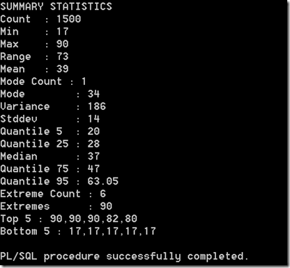
image

We can compare this to what is produced by the Explore Node in ODM

image

image

We can see that the Explore Node gives us more statistics to help us with understanding the data.

What Statistics does the Explore Node produce

We can see the actual SQL code that the Explore Node runs to get the statistics that are displayed in the Explore Node View Data window. To do this you will need to right-click on the Explore Node and move the mouse down to the Deploy option. The submenu will open and select ‘SQL to Clipboard’ from the list. Open a text editor and past the code. You  will need to tidy up some of this code to point it at the actual data source you want. You will get the following

SELECT /*+ inline */  ATTR, 
       DATA_TYPE, 
       NULL_PERCENT, 
       DISTINCT_CNT, 
       DISTINCT_PERCENT, 
       MODE_VALUE,
       AVG,
       MIN,
       MAX,
       STD,
       VAR,
       SKEWNESS,
       KURTOSIS,
       HISTOGRAMS
FROM OUTPUT_1_23;

Where OUTPUT_1_23 is a working table that ODM has created to store intermediate results from some of its processing. In this case the Explore Node. You will need to change this to the ODM working table in your schema.

This query does not perform any of the statistics gathering. It just presents the results.

Creating our own Statistics gathering script – Part 1

The attribute names in the above SQL query tells us what statistics functions within Oracle that were used. We can replicate this statistics gathering task using the following script. There are four parts to this script. The first part gathers most of the common statistics for the attribute. The second and third parts calculate the Skewness and Kurtosis for the attribute. The final (fourth) part combines the first three parts and lists the outputs.

The one statistic function that we are not including at this point is the Histogram information. I will cover this in the next (second) blog post on statistics.

The following script has the data source table/view name included (MINING_DATA_BUILD_V) and the attribute we are going to use (AGE).  You will need to modify this script to run it for each attribute.

WITH
    basic_statistics AS (select (sum(CASE WHEN age IS NULL THEN 1 ELSE 0 END)/COUNT(*))*100 null_percent,
          count(*)    num_value,
          count(distinct age)   distinct_count,
          (count(distinct age)/count(*))*100     distinct_percent,
          avg(age)      avg_value,
          min(age)      min_value,
          max(age)     max_value,
          stddev(age)  std_value,
          stats_mode(age)   mode_value,
          variance(age)       var_value
        from   mining_data_build_v),
    skewness AS (select avg(SV) S_value
                 from (select power((age - avg(age) over ())/stddev(age) over (), 3) SV
                       from mining_data_build_v) ),
    kurtosis AS (select avg(KV) K_value
                 from (select power((age - avg(age) over ())/stddev(age) over (), 4) KV
                       from mining_data_build_v) )
SELECT null_percent,
       num_value,
       distinct_percent,
       avg_value,
       min_value,
       max_value,
       std_value,
       mode_value,
       var_value,
       S_value,
       K_value
from basic_statistics,
     skewness,
     kurtosis;

image

Part 2 – Lets do it for all the attributes in a table

In the code above I’ve shown how you can gather the statistics for one particular attribute of one table.But in with an analytics project you will want to gather the statistics on all the attributes.

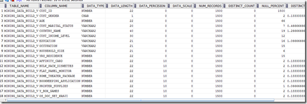
What we can do is to take the code above and put it into a procedure. This procedure accepts a table name as input, loops through the attributes for this table and calculates the various statistics. The statistics are saved in a table called DATA_STATS (see below).

drop table data_stats;

create table DATA_STATS (
table_name VARCHAR2(30) NOT NULL,
column_name VARCHAR2(30) NOT NULL,
data_type VARCHAR2(106) NOT NULL,
data_length NUMBER,
data_percision NUMBER,
data_scale NUMBER,
num_records NUMBER,
distinct_count NUMBER,
null_percent NUMBER,
distinct_percent NUMBER,
avg_value NUMBER,
min_value NUMBER,
max_value NUMBER,
std_value NUMBER,
mode_value VARCHAR2(1000),
var_value NUMBER,
s_value NUMBER,
k_value NUMBER,
PRIMARY KEY (table_name, column_name));

This is one of the first things that I do when I start on a new project. I create the DATA_STATS table and run my procedure GATHER_DATA_STATS for each table that we will be using. By doing this it allows me to have a permanent records of the stats for each attribute and saves me time in having to rerun various stats at different points of the project. I can also use these stats to produces some additional stats or to produce some graphs.

He is the code for the GATHER_DATA_STATS procedure.

CREATE OR REPLACE PROCEDURE gather_data_stats(p_table_name IN varchar2) AS

   cursor c_attributes (c_table_name varchar2)
                       is SELECT table_name,
                                 column_name,
                                 data_type,
                                 data_length,
                                 data_precision,
                                 data_scale
                          FROM user_tab_columns
                          WHERE table_name = upper(c_table_name);

   v_sql     NUMBER;
   v_rows    NUMBER;
BEGIN
   dbms_output.put_line('Starting to gather statistics for '||upper(p_table_name)||' at '||to_char(sysdate,'DD-MON-YY HH24:MI:SS'));

   FOR r_att in c_attributes(p_table_name) LOOP
      --
      -- remove any previously generated stats
      --
      v_sql := DBMS_SQL.OPEN_CURSOR;
      DBMS_SQL.PARSE(v_sql, 'delete from DATA_STATS where table_name = '''||r_att.table_name||''' and column_name = '''||r_att.column_name||'''', DBMS_SQL.NATIVE);
      v_rows := DBMS_SQL.EXECUTE(v_sql);
--dbms_output.put_line('delete from DATA_STATS where table_name = '''||r_att.table_name||''' and column_name = '''||r_att.column_name||'''');

      IF r_att.data_type = 'NUMBER' THEN
         dbms_output.put_line(r_att.table_name||' : '||r_att.column_name||' : '||r_att.data_type);

         --
         -- setup the insert statement and execute
         --
         v_sql := DBMS_SQL.OPEN_CURSOR;
         DBMS_SQL.PARSE(v_sql, 'insert into data_stats select '''||r_att.table_name||''', '''||r_att.column_name||''', '''||r_att.data_type||''', '||r_att.data_length||', '||nvl(r_att.data_precision,0)||', '||nvl(r_att.data_scale,0)||', count(*) num_value, (sum(CASE WHEN '||r_att.column_name||' IS NULL THEN 1 ELSE 0 END)/COUNT(*))*100 null_percent, count(distinct '||r_att.column_name||') distinct_count, (count(distinct '||r_att.column_name||')/count(*))*100 distinct_percent, avg('||r_att.column_name||') avg_value, min('||r_att.column_name||') min_value, max('||r_att.column_name||') max_value, stddev('||r_att.column_name||') std_value, stats_mode('||r_att.column_name||') mode_value, variance('||r_att.column_name||') var_value, null, null from '|| r_att.table_name, DBMS_SQL.NATIVE);
         v_rows := DBMS_SQL.EXECUTE(v_sql);

      ELSIF r_att.data_type IN ('CHAR', 'VARCHAR', 'VARCHAR2') THEN
         dbms_output.put_line(r_att.table_name||' : '||r_att.column_name||' : '||r_att.data_type);

         --
         -- We need to gather a smaller number of stats for the character attributes
         --
         v_sql := DBMS_SQL.OPEN_CURSOR;
         begin

         DBMS_SQL.PARSE(v_sql, 'insert into data_stats select '''||r_att.table_name||''', '''||r_att.column_name||''', '''||r_att.data_type||''', '||r_att.data_length||', '||nvl(r_att.data_precision,0)||', '||nvl(r_att.data_scale,0)||', count(*) num_value, (sum(CASE WHEN '||r_att.column_name||' IS NULL THEN 1 ELSE 0 END)/COUNT(*))*100 null_percent, count(distinct '||r_att.column_name||') distinct_count, (count(distinct '||r_att.column_name||')/count(*))*100 distinct_percent, null, null, null, null, stats_mode('||r_att.column_name||') mode_value, null, null, null from '|| r_att.table_name, DBMS_SQL.NATIVE);
         v_rows := DBMS_SQL.EXECUTE(v_sql);

-- dbms_output.put_line('insert into data_stats select '''||r_att.table_name||''', '''||r_att.column_name||''', '''||r_att.data_type||''', '||r_att.data_length||', '||nvl(r_att.data_precision,0)||', '||nvl(r_att.data_scale,0)||', count(*) num_value, (sum(CASE WHEN '||r_att.column_name||' IS NULL THEN 1 ELSE 0 END)/COUNT(*))*100 null_percent, count(distinct '||r_att.column_name||') distinct_count, (count(distinct '||r_att.column_name||')/count(*))*100 distinct_percent, null, null, null, null, stats_mode('||r_att.column_name||') mode_value, null, null, null from '|| r_att.table_name);
         exception
         when others then
            dbms_output.put_line(v_rows);
         end;

      ELSE
         dbms_output.put_line('Unable to gather statistics for '||r_att.column_name||' with data type of '||r_att.data_type||'.');
      END IF;
   END LOOP;

   dbms_output.put_line('Finished gathering statistics for '||upper(p_table_name)||' at '||to_char(sysdate,'DD-MON-YY HH24:MI:SS'));
  
   commit;
END;

Then to run it for a table:

exec gather_data_stats('mining_data_build_v');

We can view the contents of the DATA_STATS table by executing the following in SQL*Plus or SQL Developer

select * from DATA_STATS;
image