Showing posts with label Oracle. Show all posts

Wednesday, April 24, 2019

Time Series Forecasting in Oracle – Part 2

This is the second part about time-series data modeling using Oracle. Check out the first part here.

In this post I will take a time-series data set and using the in-database time-series functions model the data, that in turn can be used for predicting future values and trends.

The data set used in these examples is the Rossmann Store Sales data set. It is available on Kaggle and was used in one of their competitions.

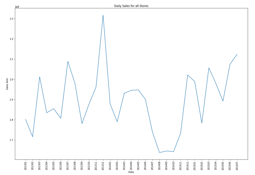
Let's start by aggregating the data to monthly level. We get.
Screenshot 2019-04-16 12.37.59  

Data Set-up
Although not strictly necessary, but it can be useful to create a subset of your time-series data to only contain the time related attribute and the attribute containing the data to model. When working with time-series data, the exponential smoothing function expects the time attribute to be of DATE data type. In most cases it does. When it is a DATE, the function will know how to process this and all you need to do is to tell the function the interval. A view is created to contain the monthly aggregated data.

-- Create input time series
create or replace view demo_ts_data as 
select to_date(to_char(sales_date, 'MON-RRRR'),'MON-RRRR') sales_date,
sum(sales_amt) sales_amt
from demo_time_series
group by to_char(sales_date, 'MON-RRRR')
order by 1 asc;

Next a table is needed to contain the various settings for the exponential smoothing function.

CREATE TABLE demo_ts_settings(setting_name VARCHAR2(30), 
                              setting_value VARCHAR2(128));

Some care is needed with selecting the parameters and their settings as not all combinations can be used.

Example 1 - Holt-Winters
The first example is to create a Holt-Winters time-series model for hour data set. For this we need to set the parameter to include defining the algorithm name, the specific time-series model to use (exsm_holt), the type/size of interval (monthly) and the number of predictions to make into the future, pass the last data point.

BEGIN
   -- delete previous setttings
   delete from demo_ts_settings;

   -- set ESM as the algorithm
   insert into demo_ts_settings 
      values (dbms_data_mining.algo_name,
              dbms_data_mining.algo_exponential_smoothing);

   -- set ESM model to be Holt-Winters
   insert into demo_ts_settings 
      values (dbms_data_mining.exsm_model,
              dbms_data_mining.exsm_holt);

   -- set interval to be month
   insert into demo_ts_settings 
      values (dbms_data_mining.exsm_interval,
              dbms_data_mining.exsm_interval_month);

   -- set prediction to 4 steps ahead
   insert into demo_ts_settings 
      values (dbms_data_mining.exsm_prediction_step,
              '4');

   commit; 
END;

Now we can call the function, generate the model and produce the predicted values.

BEGIN
   -- delete the previous model with the same name
   BEGIN 
      dbms_data_mining.drop_model('DEMO_TS_MODEL');
   EXCEPTION 
      WHEN others THEN null; 
   END;

   dbms_data_mining.create_model(model_name => 'DEMO_TS_MODEL',
                                 mining_function => 'TIME_SERIES',
                                 data_table_name => 'DEMO_TS_DATA',
                                 case_id_column_name => 'SALES_DATE',
                                 target_column_name => 'SALES_AMT',
                                 settings_table_name => 'DEMO_TS_SETTINGS');
END;

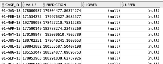
When the model is create a number of data dictionary views are populated with model details and some addition views are created specific to the model. One such view commences with DM$VP. Views commencing with this contain the predicted values for our time-series model. You need to append the name of the model create, in our example DEMO_TS_MODEL.
 
-- get predictions
select case_id, value, prediction, lower, upper 
from   DM$VPDEMO_TS_MODEL
order by case_id;


Screenshot 2019-04-16 16.01.14

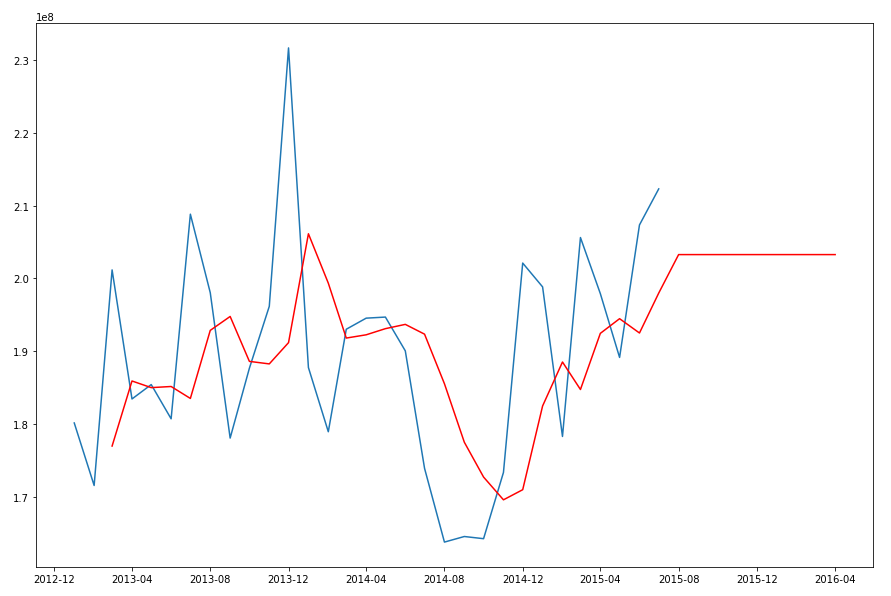
When we plot this data we get. Screenshot 2019-04-16 16.02.57 The blue line contains the original data values and the red line contains the predicted values. The predictions are very similar to those produced using Holt-Winters in Python. Screenshot 2019-04-16 16.04.45  

Example 2 - Holt-Winters including Seasonality
The previous example didn't really include seasonality int the model and predictions. In this example we introduce seasonality to allow the model to pick up any trends in the data based on a defined period. For this example we will change the model name to HW_ADDSEA, and the season size to 5 units. A data set with a longer time period would illustrate the different seasons better but this gives you an idea.

BEGIN
   -- delete previous setttings
   delete from demo_ts_settings;

   -- select ESM as the algorithm
   insert into demo_ts_settings 
   values (dbms_data_mining.algo_name,
           dbms_data_mining.algo_exponential_smoothing);

   -- set ESM model to be Holt-Winters Seasonal Adjusted
   insert into demo_ts_settings 
   values (dbms_data_mining.exsm_model,
           dbms_data_mining.exsm_HW_ADDSEA);

   -- set interval to be month
   insert into demo_ts_settings 
   values (dbms_data_mining.exsm_interval,
   dbms_data_mining.exsm_interval_month);

  -- set prediction to 4 steps ahead
  insert into demo_ts_settings 
  values (dbms_data_mining.exsm_prediction_step,
          '4');

   -- set seasonal cycle to be 5 quarters
   insert into demo_ts_settings 
   values (dbms_data_mining.exsm_seasonality,
           '5');

commit; 
END;

We need to re-run the creation of the model and produce the predicted values. This code is unchanged from the previous example.

BEGIN
   -- delete the previous model with the same name
   BEGIN 
      dbms_data_mining.drop_model('DEMO_TS_MODEL');
   EXCEPTION 
      WHEN others THEN null; 
   END;

   dbms_data_mining.create_model(model_name => 'DEMO_TS_MODEL',
                                 mining_function => 'TIME_SERIES',
                                 data_table_name => 'DEMO_TS_DATA',
                                 case_id_column_name => 'SALES_DATE',
                                 target_column_name => 'SALES_AMT',
                                 settings_table_name => 'DEMO_TS_SETTINGS');
END;

When we re-query the DM$VPDEMO_TS_MODEL we get the new values. When plotted we get. Screenshot 2019-04-16 16.17.30
The blue line contains the original data values and the red line contains the predicted values.

Comparing this chart to the chart from the first example we can see there are some important differences between them. These differences are particularly evident in the second half of the chart, on the right hand side. We get to see there is a clearer dip in the predicted data. This mirrors the real data values better. We also see better predictions as the time line moves to the end.

When performing time-series analysis you really need to spend some time exploring the data, to understand what is happening, visualizing the data, seeing if you can identifying any patterns, before moving onto using the different models. Similarly you will need to explore the various time-series models available and the parameters, to see what works for your data and follow the patterns in your data. There is not magic solution in this case.

Wednesday, March 13, 2019

OCI - Making DBaaS Accessible using port 1521

When setting up a Database on Oracle Cloud Infrastructure (OCI) for the first time there are a few pre and post steps to complete before you can access the database using a JDBC type of connect, just like what you have in SQL Developer, or using Python or other similar tools and/or languages.  

1. Setup Virtual Cloud Network (VCN)
The first step, when starting off with OCI, is to create a Virtual Cloud Network.

 Screenshot 2019-03-13 11.08.48


Create a VCN and take all the defaults. But change the radio button shown in the following image.
 Screenshot 2019-03-13 11.13.07

That's it. We will come back to this later.

2. Create the Oracle Database To create the database
select 'Bare Metal, VM and Exadata' from the menu.

 Screenshot 2019-03-13 11.14.08

Click on the 'Launch DB System' button.
 Screenshot 2019-03-13 11.15.28

 Fill in the details of the Database you want to create and select from the various options from the drop-downs.
 Screenshot 2019-03-13 11.16.56
Fill in the details of the VCN you created in the previous set, and give the name of the DB and the Admin password.
 Screenshot 2019-03-13 11.19.00
When you are finished everything that is needed, the 'Launch DB System' at the bottom of the page will be enabled. After clicking on this botton, the VM will be built and should be ready in a few minutes. When finished you should see something like this.
 Screenshot 2019-03-13 11.22.51  3. SSH to the Database server
 When the DB VM has been created you can now SSH to it. You will need to use the SSH key file used when creating the DB VM. You will need to connect to the opc (operating system user), and from there sudo to the oracle user. For example
 
<ssh file> opc@<public IP address>

The public IP address can be found with the Database VM details
 
Screenshot 2019-03-13 11.26.35
[opc@tudublins1 ~]$ sudo su - oracle
[oracle@tudublins1 ~]$ . oraenv
ORACLE_SID = [cdb1] ? 
The Oracle base has been set to /u01/app/oracle
[oracle@tudublins1 ~]$ 
[oracle@tudublins1 ~]$ sqlplus / as sysdba

SQL*Plus: Release 18.0.0.0.0 - Production on Wed Mar 13 11:28:05 2019
Version 18.3.0.0.0

Copyright (c) 1982, 2018, Oracle. All rights reserved.


Connected to:
Oracle Database 18c Enterprise Edition Release 18.0.0.0.0 - Production
Version 18.3.0.0.0

SQL> alter session set container = pdb1;

Session altered.

SQL> create user demo_user identified by DEMO_user123##;

User created.

SQL> grant create session to demo_user;

Grant succeeded.

SQL>

4. Open port 1521 
To be able to access this with a Basic connection in SQL Developer and most programming languages, we will need to open port 1521 to allow these tools and languages to connect to the database. To do this go back to the Virtual Cloud Networks section from the menu.

Screenshot 2019-03-13 11.08.48

Click into your VCN, that you created earlier. You should see something like the following.

Screenshot 2019-03-13 11.34.53

Click on the Security Lists, menu option on the left hand side.

Screenshot 2019-03-13 11.39.10
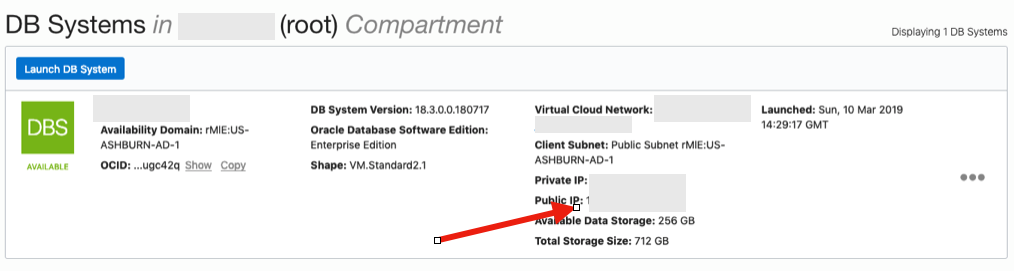
From that screen, click on Default Security List, and then click on the 'Edit All Rules' button at the top of the next screen. Add a new rule to have a 'Destination Port Range' set for 1521
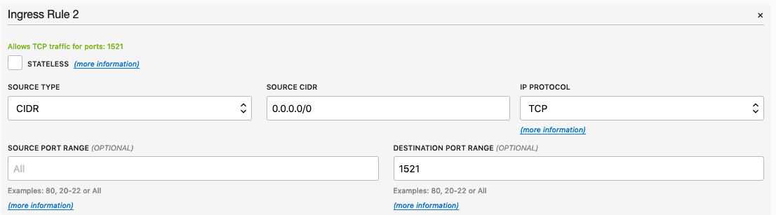
Screenshot 2019-03-13 11.41.19

That's it.

 5. Connect to the Database from anywhere

Now you can connect to the OCI Database using a basic SQL Developer Connection.


Screenshot 2019-03-13 11.46.06

Monday, February 4, 2019

Machine Learning Models in Python - How long does it take

We keep hearing from people about all the computing resources needed for machine learning. Sometimes it can put people off from trying it as they will think I don't have those kind of resources.

This is another blog post in my series on 'How long does it take to create a machine learning model?'

Check out my previous blog post that used data sets containing 72K, 210K, 660K, 2M and 10M records.
There was some surprising results in those these.

In this test, I'll be using Python and SciKitLearn package to create models using the same algorithms. There are a few things to keep in mind. Firstly, although they maybe based on the same algorithms, the actual implementation of them will be different in each environment (SQL vs Python).

With using Python for machine learning, one of the challenges we have is getting access to the data. Assuming the data lives in a Database then time is needed to extract that data to the local Python environment. Secondly, when using Python you will be using a computer with significantly less computing resources than a Database server. In this test I used my laptop (MacBook Pro). Thirdly, when extracting the data from the database, what method should be used.

I've addressed these below and the Oracle Database I used was the DBaaS I used in my first experiment. This is a Database hosted on Oracle Cloud.

Extracting Data to CSV File
This kind of depends on how you do this. There are hundreds of possibilities available to you, but if you are working with an Oracle Database you will probably be using SQL Developer. I used the 'export' option to create a CSV file for each of the data sets. The following table shows how long it took for each data set.

As you can see this is an incredibly slow way of exporting this data. Like I said, there are quicker ways of doing this.

After downloading the data sets, the next step is to see how load it takes to load these CSV files into a pandas data frame in Python. The following table show the timings in seconds.


You can see that Python is very efficient at loading these data sets into a pandas data frame in my Python environment.

Extracting Data using cx_Oracle Python package
As I'll be using Python to create the models and the data exists in an Oracle Database (on Oracle Cloud), I can use the cx_Oracle package to download the data sets into my Python environment. After using the cx_Oracle package to download the data I then converted it into a pandas data frame.


You can see that using cx_Oracle to download the data is a very efficient way of accessing the data.  But if the data already exists in CSV files, then the previous method would be quicker to use.

I had the array fetch size set to 10,000.  I also experimented with smaller and larger numbers for the array fetch size, but 10,000 seemed to give a quickest results.

How long to create Machine Learning Models in Python
Now we get onto checking out the timings of how long it takes to create a number of machine learning models using different algorithms and using the default settings. The algorithms include Naive Bayes, Decision Tree, GLM, SVM and Neural Networks.


I had to stop including SVM in the tests as it was taking way too long to run. For example I killed the SVM model build on the 210K data set after it was running for 5 hours.

The Neural Network models created had 3 hidden layers.

In addition to creating the models, there was some minor data preparation steps performed including factorizing, normalization and one-hot-coding. This data preparation would be comparable to the automatic data preparation steps performed by Oracle, although Oracle Automatic Data Preparation does a bit of extra work.


At the point I would encourage you to look back at my previous blog posts on timings using Oracle DBaaS and ADW.  You will see that Python, in these test cases, was quicker at creating the machine learning models. But with Python the data needed to be extracted from the database and that can take time!

A separate consideration is being able to deploy the models. The time it takes to build models is perhaps not the main consideration. You need to consider ease of deployment and use of the models.

Wednesday, August 29, 2018

Bringing Neural Networks to Production using GraphPipe

Machine learning is a fascinating topic. It has so much potential yet very few people talk about using machine learning in production. I've been highlighting the need for this for over 20 years now and only a very small number of machine learning languages and solutions are suitable for production use. Why? maybe it is due to the commercial aspects and as many of the languages and tools are driven by the open source community, one of the last things they get round to focusing on is production deployment. Rightly they are focused at developing more and more machine learning algorithms and features for developing models, but where the real value comes is will being able to embed machine learning model scoring in production system. Maybe this why the dominant players with machine learning in enterprises are still the big old analytics companies.

Yes that was a bit a of a rant but it is true. But over the summer and past few months there has been a number of articles about production deployment.

But this is not a new topic. For example, we have Predictive Model Markup Language (PMML) around for a long time. The aim of this was to allow the interchange of models between different languages. This would mean that the data scientist could develop their models using one language and then transfer or translate the model into another language that offers the same machine learning algorithms.

But the problem with this approach is that you may end up with different results being generated by the model in the development or lab environment versus the model being used in production. Why does this happen? Well the algorithms are developed by different people/companies and everyone has their preferences for how these algorithms are implemented.

To over come this some companies would rewrite their machine learning algorithms and models to ensure that development/lab results matched the results in production. But there is a very large cost associated with this development and ongoing maintenance as the models evolved. This would occur, maybe, every 3, 6, 9, 12 months. Somethings the time to write or rewrite each new version of the model would be longer than its lifespan.

These kind of problems have been very common and has impacted on model deployment in production.

In the era of cloud we are now seeing some machine learning cloud solutions making machine learning models available using REST services. These can, very easily, allow for machine learning models to be included in production applications. You are going to hear more about this topic over the coming year.

But, despite all the claims and wonders and benefits of cloud solutions, it isn't for everyone. Maybe at some time in the future but it mightn't be for some months or years to come.

So, how can we easily add machine learning model scoring/labeling to our production systems? Well we need some sort of middleware solutions.

Given the current enthusiasm for neural networks, and the need for GPUs, means that these cannot (easily) be deployed into production applications.

There have been some frameworks put forward for how to enable this. Once such framework is called Graphpipe. This has recently been made open source by Oracle.

Graphpipe

Graphpipe is a framework that to access and use machine learning models developed and running on different platforms. The framework allows you to perform model scoring across multiple neural networks models and create ensemble solutions based on these. Graphpipe development has been focused on performance (most other frameworks don't). It uses flatbuffers for efficient transfer of data and currently has integration with TensorFlow, PyTorch, MXNet, CNTK and via ONNX and caffe2.

Expect to have more extensions added to the framework.

Graphpipe website

Graphpipe getting started

Graphpipe blogpost

Graphpipe download

Monday, June 18, 2018

Twitter Analytics using Python - Part 3

This is my third (of five) post on using Python to process Twitter data.

Check out my all the posts in the series.

In this post I'll have a quick look at how to save the tweets you have download. By doing this allows you to access them at a later point and to perform more analysis. You have a few instances of saving the tweets. The first of these is to save them to files and the second option is to save them to a table in a database.

Saving Tweets to files

In the previous blog post (in this series) I had converged the tweets to Pandas and then used the panda structure to perform some analysis on the data and create some charts. We have a very simple command to save to CSV.

# save tweets to a file
tweets_pd.to_csv('/Users/brendan.tierney/Dropbox/tweets.csv', sep=',')

We can inspect this file using a spreadsheet or some other app that can read CSV files and get the following.

Twitter app8

When you want to read these tweets back into your Python environment, all you need to do is the following.

# and if we want to reuse these tweets at a later time we can reload them
old_tweets = pd.read_csv('/Users/brendan.tierney/Dropbox/tweets.csv')

old_tweets

Tweet app9

That's all very easy!


Saving Tweets to a Database

There are two ways to add tweets to table in the database. There is the slow way (row-by-row) or the fast way doing a bulk insert.

Before we get started with inserting data, lets get our database connection setup and the table to store the tweets for our date. To do this we need to use the cx_oracle python library. The following codes shows the setting up of the connections details (without my actual login details), establishes the connects and then retrieves some basic connection details to prove we are connected.

# import the Oracle Python library
import cx_Oracle

# define the login details
p_username = "..."
p_password = "..."
p_host = "..."
p_service = "..."
p_port = "1521"

# create the connection
con = cx_Oracle.connect(user=p_username, password=p_password, dsn=p_host+"/"+p_service+":"+p_port)
cur = con.cursor()

# print some details about the connection and the library
print("Database version:", con.version)
print("Oracle Python version:", cx_Oracle.version)


Database version: 12.1.0.1.0
Oracle Python version: 6.3.1

Now we can create a table based on the current date.

# drop the table if it already exists
#drop_table = "DROP TABLE TWEETS_" + cur_date
#cur.execute(drop_table)

cre_table = "CREATE TABLE TWEETS_" + cur_date + " (tweet_id number, screen_name varchar2(100), place varchar2(2000), lang varchar2(20), date_created varchar2(40), fav_count number, retweet_count number, tweet_text varchar2(200))"

cur.execute(cre_table)

Now lets first start with the slow (row-by-row) approach. To do this we need to take our Panda data frame and convert it to lists that can be indexed individually.

lst_tweet_id = [item[0] for item in rows3]
lst_screen_name = [item[1] for item in rows3]
lst_lang =[item[3] for item in rows3]
lst_date_created = [item[4] for item in rows3]
lst_fav_count = [item[5] for item in rows3]
lst_retweet_count = [item[6] for item in rows3]
lst_tweet_text = [item[7] for item in rows3]

#define a cursor to use for the the inserts
cur = con.cursor()
for i in range(len(rows3)):
    #do the insert using the index. This can be very slow and should not be used on big data
    cur3.execute("insert into TWEETS_2018_06_12 (tweet_id, screen_name, lang, date_created, fav_count, retweet_count, tweet_text) values (:arg_1, :arg_2, :arg_3, :arg_4, :arg_5, :arg_6, :arg_7)",
                 {'arg_1':lst_tweet_id[i], 'arg_2':lst_screen_name[i], 'arg_3':lst_lang[i], 'arg_4':lst_date_created[i],
                  'arg_5':lst_fav_count[i], 'arg_6':lst_retweet_count[i], 'arg_7':lst_tweet_text[i]})

#commit the records to the database and close the cursor
con.commit()
cur.close()

Tweet app10

Now let us look a quicker way of doing this.

WARNING: It depends on the version of the cx_oracle library you are using. You may encounter some errors relating to the use of floats, etc. You might need to play around with the different versions of the library until you get the one that works for you. Or these issues might be fixed in the most recent versions.

The first step is to convert the panda data frame into a list.

rows = [tuple(x) for x in tweets_pd.values]
rows

Tweet app11

Now we can do some cursor setup like setting the array size. This determines how many records are sent to the database in each batch. Better to have a larger number than a single digit number.

cur = con.cursor()

cur.bindarraysize = 100

cur2.executemany("insert into TWEETS_2018_06_12 (tweet_id, screen_name, place, lang, date_created, fav_count, retweet_count, tweet_text) values (:1, :2, :3, :4, :5, :6, :7, :8)", rows)

Check out the other blog posts in this series of Twitter Analytics using Python.

Monday, March 12, 2018

Oracle Code Presentation March 2018

Last week I was presenting at Oracle Code in New York. I've presented at a few Oracle Code events over the past 12 months and it is always interesting to meet and talk with developers from around the World.

The title of my presentation this time was 'SQL: The one language to rule all your data'.

I've given this presentation a few times at different events (POUG, OOW, Oracle Code). I take the contents of this presentation for granted and that most people know these things. But the opposite is true. Well a lot of people do know these things, but a magnitude more do not seem to know.

For example, at last weeks Oracle Code event, I had about 100 people in the room. I started out by asking the attendees 'How many of you write SQL every day?'. About 90% put up their hand. Then a few minutes later after I start talking about various statistical functions in the database, I then ask them to 'Count how many statistical functions they have used?' I then asked them to raise their hands if they use over five statistical functions. About eight people put up their hands. Then I asked how many people use over ten functions. To my surprise only one (yes one) person put up their hand.

The feedback from the attendees was fantastic and they were very eager to go back to their day jobs and start implementing better SQL code and to learn more about the database. All they have to do is to send me 15% of their pay rises (a bit of a joke during the presentation. You had to be there ...)

The first half of the presentation talks about statistical, analytical and machine learning in the database.

The second half covers some (not all) of the various data types and locations of data that can be accessed from the database.

The presentation then concludes with the title of the presentation about SQL being the one language to rule all your data.

Based on last weeks experience, it looks like a lot more people need to hear it !

Hopefully I'll get the chance to share this presentation with other events and Oracle User Group conferences.

Two of the key take away messages are:

  • Google makes us stupid
  • We need to RTFM more often

Here is a link to the slides on SlideShare

And I recorded a short video about the presentation with Bob from OTN/ODC.

Monday, March 5, 2018

Python and Oracle : Fetching records and setting buffer size

If you used other languages, including Oracle PL/SQL, more than likely you will have experienced having to play buffering the number of records that are returned from a cursor. Typically this is needed when you are processing more than a few hundred records. The default buffering size is relatively small and by increasing the size of the number of records to be buffered can dramatically improve the performance of your code.

As with all things in coding and IT, the phrase "It Depends" applies here and changing the buffering size may not be what you need and my not help you to gain optimal performance for your code.

There are lots and lots of examples of how to test this in PL/SQL and other languages, but what I'm going to show you here in this blog post is to change the buffering size when using Python to process data in an Oracle Database using the Oracle Python library cx_Oracle.

Let us begin with taking the defaults and seeing what happens. In this first scenario the default buffering is used. Here we execute a query and the process the records in a FOR loop (yes these is a row-by-row, slow-by-slow approach.

import time

i = 0
# define a cursor to use with the connection
cur2 = con.cursor()
# execute a query returning the results to the cursor
print("Starting cursor at", time.ctime())
cur2.execute('select * from sh.customers')
print("Finished cursor at", time.ctime())

# for each row returned to the cursor, print the record
print("Starting for loop", time.ctime())
t0 = time.time()
for row in cur2:
    i = i+1
    if (i%10000) == 0:
        print(i,"records processed", time.ctime())

              
t1 = time.time()
print("Finished for loop at", time.ctime())
print("Number of records counted = ", i)

ttime = t1 - t0
print("in ", ttime, "seconds.")

This gives us the following output.

Starting cursor at  10:11:43
Finished cursor at  10:11:43
Starting for loop  10:11:43
10000 records processed  10:11:49
20000 records processed  10:11:54
30000 records processed  10:11:59
40000 records processed  10:12:05
50000 records processed  10:12:09
Finished for loop at  10:12:11 
Number of records counted =  55500
in  28.398550033569336 seconds.

Processing the data this way takes approx. 28 seconds and this corresponds to the buffering of approx 50-75 records at a time. This involves many, many, many round trips to the the database to retrieve this data. This default processing might be fine when our query is only retrieving a small number of records, but as our data set or results set from the query increases so does the time it takes to process the query.

But we have a simple way of reducing the time taken, as the number of records in our results set increases. We can do this by increasing the number of records that are buffered. This can be done by changing the size of the 'arrysize' for the cursor definition. This reduces the number of "roundtrips" made to the database, often reducing networks load and reducing the number of context switches on the database server.

The following gives an example of same code with one additional line.

cur2.arraysize = 500

Here is the full code example.

# Test : Change the arraysize and see what impact that has
import time

i = 0
# define a cursor to use with the connection
cur2 = con.cursor()
cur2.arraysize = 500
# execute a query returning the results to the cursor
print("Starting cursor at", time.ctime())
cur2.execute('select * from sh.customers')
print("Finished cursor at", time.ctime())

# for each row returned to the cursor, print the record
print("Starting for loop", time.ctime())
t0 = time.time()
for row in cur2:
    i = i+1
    if (i%10000) == 0:
        print(i,"records processed", time.ctime())

              
t1 = time.time()
print("Finished for loop at", time.ctime())
print("Number of records counted = ", i)

ttime = t1 - t0
print("in ", ttime, "seconds.")

Now the response time to process all the records is.

Starting cursor at 10:13:02 Finished cursor at 10:13:02 Starting for loop 10:13:02 10000 records processed 10:13:04 20000 records processed 10:13:06 30000 records processed 10:13:08 40000 records processed 10:13:10 50000 records processed 10:13:12 Finished for loop at 10:13:13 Number of records counted = 55500 in 11.780734777450562 seconds.

All done in just under 12 seconds, compared to 28 seconds previously.

Here is another alternative way of processing the data and retrieves the entire results set, using the 'fetchall' command, and stores it located in 'res'.

# Test : Change the arraysize and see what impact that has
import time

i = 0
# define a cursor to use with the connection
cur2 = con.cursor()
cur2.arraysize = 500
# execute a query returning the results to the cursor
print("Starting cursor at", time.ctime())
cur2.execute('select * from sh.customers')

t0 = time.time()
print("starting FetchAll at", time.ctime())
res = cur2.fetchall()
              
t1 = time.time()
print("finished FetchAll at", time.ctime())

ttime = t1 - t0
print("in ", ttime, "seconds.")

Friday, March 2, 2018

Oracle 18c DBaaS Cloud Setup

The 18c Oracle DBaaS is now available. This is the only place that Oracle 18c will be available until later in 2018. So if you want to try it out, then you are going to need to get some Oracle Cloud credits, or you may already have a paying account for Oracle Cloud.

NewImage

The following outlines the steps you need to go through to gets Oracle 18c setup.

1. Log into your Oracle Cloud

Log into your Oracle Cloud environment. Depending on your access path you will get to your dashboard.

Select Create Instance from the dashboard.

NewImage

2. Create a new Database

From the list of services to create, select Database.

NewImage

3. Click 'Create Instance'

NewImage

4. Enter the Database Instance details

Enter the details for your new Oracle 18c Database. I've called mine 'db18c'.

Then for the Software Release dropdown list, select 'Oracle Database 18c'.

Next select the Software Edition from the dropdown list.

NewImage

5. Fill in the Instance Details

Fill in the details for 'DB Name', 'PDB Name', 'Administration Password', 'Confirm Password', setup the SSH Public Key, and then decide if you need the Backup and Recovery option.

NewImage<

6. Create the DBaaS

Double check everything and when ready click on the 'Create' button.

NewImage

7. Wait for Everything to be Create

Now is the time to be patient and wait while your cloud service is created.

NewImage

I've created two different version of the 18c Oracle DBaaS. The Enterprise Edition to 30 minutes to complete and the High Performance service too 47 minutes.

No it's time to go play.

Sunday, February 18, 2018

18c is now available (but only on the Cloud)

On Friday afternoon (16th February) we started to see tweets and blog posts from people in Oracle saying that Oracle 18c was now available. But is only available on Oracle Cloud and Engineered Systems.

It looks like we will have to wait until the Autumn before we can install it ourselves on our own servers :-(

Here is the link to the official announcement for Oracle 18c.

Oracle 18c is really Oracle 12.2.0.2. The next full new release of the Oracle database is expected to be Oracle 19.

The new features and incremental enhancements in Oracle 18c are:

  • Multitenant
  • In-Memory
  • Sharding
  • Memory Optimized Fetches
  • Exadata RAC Optimizations
  • High Availability
  • Security
  • Online Partition Merge
  • Improved Machine Learning (OAA)
  • Polymorphic Table Functions
  • Spatial and Graph
  • More JSON improvements
  • Private Temporary Tablespaces
  • New mode for Connection Manager

And now the all important links to the documentation.

Oracle 18c Documentation

Oracle 18c New Features

Oracle 18c Data Warehousing

To give Oracle 18c a try you will need to go to cloud.oracle.com and select Database from the drop down list from the Platform menu. Yes you are going to need an Oracle Cloud account and some money or some free credit. Go and get some free cloud credits at the upcoming Oracle Code events.

If you want a 'free' way of trying out Oracle 18c, you can use Oracle Live SQL. They have setup some examples of the new features for you to try.

NewImage

NOTE: Oracle 18c is not Autonomous. Check out Tim Hall's blog posts about this. The Autonomous Oracle Database is something different, and we will be hearing more about this going forward.

Tuesday, February 13, 2018

Oracle and Python setup with cx_Oracle

Is Python the new R?

Maybe, maybe not, but that I'm finding in recent months is more companies are asking me to use Python instead of R for some of my work.

In this blog post I will walk through the steps of setting up the Oracle driver for Python, called cx_Oracle. The documentation for this drive is good and detailed with plenty of examples available on GitHub. Hopefully there isn't anything new in this post, but it is my experiences and what I did.

1. Install Oracle Client
The Python driver requires Oracle Client software to be installed. Go here, download and install. It's a straightforward install. Make sure the directories are added to the search path.

2. Download and install cx_Oracle
You can use pip3 to do this.
 
pip3 install cx_Oracle

Collecting cx_Oracle
  Downloading cx_Oracle-6.1.tar.gz (232kB)
    100% |████████████████████████████████| 235kB 679kB/s
Building wheels for collected packages: cx-Oracle
  Running setup.py bdist_wheel for cx-Oracle ... done
  Stored in directory: /Users/brendan.tierney/Library/Caches/pip/wheels/0d/c4/b5/5a4d976432f3b045c3f019cbf6b5ba202b1cc4a36406c6c453
Successfully built cx-Oracle
Installing collected packages: cx-Oracle
Successfully installed cx-Oracle-6.1  

3. Create a connection in Python
Now we can create a connection. When you see some text enclosed in angled brackets <>, you will need to enter your detailed for your schema and database server.
 
# import the Oracle Python library
import cx_Oracle

# define the login details
p_username = ""
p_password = ""
p_host = ""
p_service = ""
p_port = "1521"

# create the connection
con = cx_Oracle.connect(user=p_username, password=p_password, dsn=p_host+"/"+p_service+":"+p_port)

# an alternative way to create the connection
# con = cx_Oracle.connect('/@/:1521')

# print some details about the connection and the library
print("Database version:", con.version)
print("Oracle Python version:", cx_Oracle.version)


Database version: 12.1.0.1.0
Oracle Python version: 6.1

4. Query some data and return results to Python
In this example the query returns the list of tables in the schema.
 
# define a cursor to use with the connection
cur = con.cursor()
# execute a query returning the results to the cursor
cur.execute('select table_name from user_tables')
# for each row returned to the cursor, print the record
for row in cur:
    print("Table: ", row)

Table:  ('DECISION_TREE_MODEL_SETTINGS',)
Table:  ('INSUR_CUST_LTV_SAMPLE',)
Table:  ('ODMR_CARS_DATA',)

Now list the Views available in the schema.
 
# define a second cursor
cur2 = con.cursor()
# return the list of Views in the schema to the cursor
cur2.execute('select view_name from user_views')
# display the list of Views
for result_name in cur2:
    print("View: ", result_name)

View:  ('MINING_DATA_APPLY_V',)
View:  ('MINING_DATA_BUILD_V',)
View:  ('MINING_DATA_TEST_V',)
View:  ('MINING_DATA_TEXT_APPLY_V',)
View:  ('MINING_DATA_TEXT_BUILD_V',)
View:  ('MINING_DATA_TEXT_TEST_V',)

5. Query some data and return to a Panda in Python
Pandas are commonly used for storing, structuring and processing data in Python, using a data frame format. The following returns the results from a query and stores the results in a panda.
 
# in this example the results of a query are loaded into a Panda
# load the pandas library
import pandas as pd

# execute the query and return results into the panda called df
df = pd.read_sql_query("SELECT * from INSUR_CUST_LTV_SAMPLE", con)

# print the records returned by query and stored in panda
print(df.head())

 CUSTOMER_ID     LAST    FIRST STATE     REGION SEX    PROFESSION  \
0     CU13388     LEIF   ARNOLD    MI    Midwest   M        PROF-2   
1     CU13386     ALVA   VERNON    OK    Midwest   M       PROF-18   
2      CU6607   HECTOR  SUMMERS    MI    Midwest   M  Veterinarian   
3      CU7331  PATRICK  GARRETT    CA       West   M       PROF-46   
4      CU2624  CAITLYN     LOVE    NY  NorthEast   F      Clerical   

  BUY_INSURANCE  AGE  HAS_CHILDREN   ...     MONTHLY_CHECKS_WRITTEN  \
0            No   70             0   ...                          0   
1            No   24             0   ...                          9   
2            No   30             1   ...                          2   
3            No   43             0   ...                          4   
4            No   27             1   ...                          4   

   MORTGAGE_AMOUNT  N_TRANS_ATM  N_MORTGAGES  N_TRANS_TELLER  \
0                0            3            0               0   
1             3000            4            1               1   
2              980            4            1               3   
3                0            2            0               1   
4             5000            4            1               2   

  CREDIT_CARD_LIMITS  N_TRANS_KIOSK  N_TRANS_WEB_BANK       LTV  LTV_BIN  
0               2500              1                 0  17621.00   MEDIUM  
1               2500              1               450  22183.00     HIGH  
2                500              1               250  18805.25   MEDIUM  
3                800              1                 0  22574.75     HIGH  
4               3000              2              1500  17217.25   MEDIUM  

[5 rows x 31 columns]

6. Wrapping it up and closing things
Finally we need to wrap thing up and close our cursors and our connection to the database.
 
# close the cursors
cur2.close()
cur.close()

# close the connection to the database
con.close()

Useful links
cx_Oracle website
cx_Oracle documentation
cx_Oracle examples on GitHub

Watch out for more blog posts on using Python with Oracle, Oracle Data Mining and Oracle R Enterprise.

Monday, December 11, 2017

Oracle Code Online December 2017

This week Oracle Code will be having an online event consisting of 5 tracks and with 3 presentations on each track. This online Oracle Code event will be given in 3 different geographic regions on 12th, 13th and 14th December. NewImage I've been selected to give one of these talks, and I've given this talk at some live Oracle Code events and at JavaOne back in October. The present is pre-recorded and I recorded this video back in September. I hope to be online at the end of some of these presentations to answer any questions, but unfortunately due to changes with my work commitments I may not be able to be online for all of them. The moderator for these events will take your questions (or you can send them to me here) and I will write a blog post answering all your questions.

Tuesday, September 19, 2017

My Oracle Open World 2017 Presentations

Oracle Open World 2017 will be happening very soon (1st-5th October). Still lots to do before I can get on that plane to San Francisco.

This year I'll be giving 2 presentations (see table below). One on the Sunday during the User Groups Sunday sessions. I've been accepted on the EMEA track. I then get a few days off to enjoy and experience OOW until Thursday when I have my second presentation that is part of JavaOne (I think!)

My OOW kicks off on Friday 29th September with the ACE Director briefing at Oracle HQ, after flying to SFO on Thursday 28th. This year it is only for one day instead of two days. I really enjoy this event as we get to learn and see what Oracle will be announcing at OOW as well as some things that will be coming out during the following few months.

DayTimePresentationLocation
Sunday13:45-14:30SQL: One Language to Rule All Your Data [OOW SUN1238]

SQL is a very powerful language that has been in use for almost 40 years. SQL comes with many powerful techniques for analyzing your data, and you can analyze data outside the database using SQL as well. Using the new Oracle Big Data SQL it is now possible to analyze data that is stored in a database, in Hadoop, and in NoSQL all at the same time. This session explores the capabilities in Oracle Database that allow you to work with all your data. Discover how SQL really is the unified language for processing all your data, allowing you to analyze, process, run machine learning, and protect all your data.

Hopefully this presentation will be a bit of Fun! For those who have been working with the database for a long time, we can sometimes forget what we can really do. For those starting out in the career may not realise what the database can do. The presentation delivers an important message while having a laugh or two (probably at me).

Marriott Marquis (Golden Gate Level) - Golden Gate C1/C2
Thursday13:45-14:30Is SQL the Best Language for Statistics and Machine Learning?

[OOW and JavaOne CON7350]

Did you know that Oracle Database comes with more than 300 statistical functions? And most of these statistical functions are available in all versions of Oracle Database? Most people do not seem to know this. When we hear about people performing statistical analytics, we hear them talking about Excel and R, but what if we could do statistical analysis in the database without having to extract any data onto client machines? This presentation explores the various statistical areas available in Oracle Database and gives several demonstrations. We can also greatly expand our statistical capabilities by using Oracle R Enterprise with the embedded capabilities in SQL.

This presentation is just one of the 14 presentations that are scheduled for the Thursday! I believe this session is already fully booked, but you can still add yourself to the wait list.

Marriott Marquis (Golden Gate Level) - Golden Gate B

My flights and hotel have been paid by OTN as part of the Oracle ACE Director program. Yes this costs a lot of money and there is no way I'd be able to pay these costs. Thank you.

My diary for OOW is really full. No it is completely over booked. It is just mental. Between attending conference session, meeting with various product teams (we only get to meet at OOW), attending various community meet-ups, this year I get to attend some events for OUG leaders (representing UKOUG), spending some time on the EMEA User Group booth, various meetings with people to discuss how they can help or contribute to the UKOUG, then there is Oak Table World, trying to check out the exhibition hall, spend some time at the OTN/ODC hangout area, getting a few OTN t-shirts, doing some book promotions at the Oracle Press shop, etc., etc., etc. I'm exhausted just thinking about it. Mosts days start at 7am and then finish around 10pm.

I'll need a holiday when I get home! but it will be straight back to work :-(

If you are at OOW and want to chat then contact me via DM on Twitter or WhatsApp (these two are best) or via email (this will be the slowest way).

I'll have another blog post listing the presentations from various people and partners from the Republic of Ireland who are speaking at OOW.

Tuesday, July 5, 2016

Cluster Distance using SQL with Oracle Data Mining - Part 4

This is the fourth and last blog post in a series that looks at how you can examine the details of predicted clusters using Oracle Data Mining. In the previous blog posts I looked at how to use CLUSER_ID, CLUSTER_PROBABILITY and CLUSTER_SET.

In this blog post we will look at CLUSTER_DISTANCE. We can use the function to determine how close a record is to the centroid of the cluster. Perhaps we can use this to determine what customers etc we might want to focus on most. The customers who are closest to the centroid are one we want to focus on first. So we can use it as a way to prioritise our workflows, particularly when it is used in combination with the value for CLUSTER_PROBABILITY.

Here is an example of using CLUSTER_DISTANCE to list all the records that belong to Cluster 14 and the results are ordered based on closeness to the centroid of this cluster.

SELECT customer_id, 
       cluster_probability(clus_km_1_37 USING *) as cluster_Prob,
       cluster_distance(clus_km_1_37 USING *) as cluster_Distance
FROM   insur_cust_ltv_sample
WHERE   cluster_id(clus_km_1_37 USING *) = 14
order by cluster_Distance asc;

Here is a subset of the results from this query.

NewImage

When you examine the results you may notice that the records that is listed first and closest record to the centre of cluster 14 has a very low probability. You need to remember that we are working in a N-dimensional space here. Although this first record is closest to the centre of cluster 14 it has a really low probability and if we examine this record in more detail we will find that it is at an overlapping point between a number of clusters.

This is why we need to use the CLUSTER_DISTANCE and CLUSTER_PROBABILITY functions together in our workflows and applications to determine how we need to process records like these.

Thursday, June 23, 2016

Cluster Sets using SQL with Oracle Data Mining - Part 3

This is the third blog post on my series on examining the Clusters that were predicted by an Oracle Data Mining model. Check out the previous blog posts.

In the previous posts we were able to list the predicted cluster for each record in our data set. This is the cluster that the records belonged to the most. I also mentioned that a record could belong to many clusters.

So how can you list all the clusters that the a record belongs to?

You can use the CLUSTER_SET SQL function. This will list the Cluster Id and a probability measure for each cluster. This function returns a array consisting of the set of all clusters that the record belongs to.

The following example illustrates how to use the CLUSTER_SET function for a particular cluster model.

SELECT t.customer_id, s.cluster_id, s.probability
FROM   (select customer_id, cluster_set(clus_km_1_37 USING *) as Cluster_Set
        from   insur_cust_ltv_sample 
        WHERE  customer_id in ('CU13386', 'CU100')) T,
      TABLE(T.cluster_set) S
order by t.customer_id, s.probability desc; 

The output from this query will be an ordered data set based on the customer id and then the clusters listed in descending order of probability. The cluster with the highest probability is what would be returned by the CLUSTER_ID function. The output from the above query is shown below.

NewImage

If you would like to see the details of each of the clusters and to examine the differences between these clusters then you will need to use the CLUSTER_DETAILS function (see previous blog post).

You can specify topN and cutoff to limit the number of clusters returned by the function. By default, both topN and cutoff are null and all clusters are returned.

- topN is the N most probable clusters. If multiple clusters share the Nth probability, then the function chooses one of them.

- cutoff is a probability threshold. Only clusters with probability greater than or equal to cutoff are returned. To filter by cutoff only, specify NULL for topN.

You may want to use these individually or combined together if you have a large number of customers. To return up to the N most probable clusters that are greater than or equal to cutoff, specify both topN and cutoff.

The following example illustrates using the topN value to return the top 4 clusters.

SELECT t.customer_id, s.cluster_id, s.probability
FROM   (select customer_id, cluster_set(clus_km_1_37, 4, null USING *) as Cluster_Set
        from   insur_cust_ltv_sample 
        WHERE  customer_id in ('CU13386', 'CU100')) T,
      TABLE(T.cluster_set) S
order by t.customer_id, s.probability desc;

and the output from this query shows only 4 clusters displayed for each record.

NewImage

Alternatively you can select the clusters based on a cut off value for the probability. In the following example this is set to 0.05.

SELECT t.customer_id, s.cluster_id, s.probability
FROM   (select customer_id, cluster_set(clus_km_1_37, NULL, 0.05 USING *) as Cluster_Set
        from   insur_cust_ltv_sample 
        WHERE  customer_id in ('CU13386', 'CU100')) T,
      TABLE(T.cluster_set) S
order by t.customer_id, s.probability desc;

and the output this time looks a bit different.

NewImage

Finally, yes you can combine these two parameters to work together.

SELECT t.customer_id, s.cluster_id, s.probability FROM (select customer_id, cluster_set(clus_km_1_37, 2, 0.05 USING *) as Cluster_Set from insur_cust_ltv_sample WHERE customer_id in ('CU13386', 'CU100')) T, TABLE(T.cluster_set) S order by t.customer_id, s.probability desc;

Thursday, June 16, 2016

Cluster Details with Oracle Data Mining - Part 2

This is the second blog post of my series on examining the clusters that are predicted for by an Oracle Data Mining model for your data. In my previous blog post I should you how to use CLUSTER_ID and CLUSTER_PROBABILITY functions. These are the core of what you will be used when working with clusters and automating the process.

In this blog post I will look at what details are used by the clustering model to make the prediction. The function that you can use is called CLUSTER_DETAILS. I had an earlier blog post on using PREDICTION_DETAILS to see some of the details that are produced when performing classification.

CLUSTER_DETAILS returns the cluster details for each row in the selection. The return value is an XML string that describes the attributes of the highest probability cluster.

Here is an example of using the CLUSTER_DETAILS function in a SELECT statement.

select cluster_details(clus_km_1_37, 14 USING *) as Cluster_Details
from   insur_cust_ltv_sample 
where  customer_id = 'CU13386';

The output is an XML string and the easiest way to view this is in SQL Developer. It will list the top 5 highest weighted attributes for the cluster centroid.

NewImage NewImage

The returned attributes are ordered by weight. The weight of an attribute expresses its positive or negative impact on cluster assignment. A positive weight indicates an increased likelihood of assignment. A negative weight indicates a decreased likelihood of assignment. By default, CLUSTER_DETAILS returns the attributes with the highest positive weights in defending order.

Tuesday, June 7, 2016

Examining predicted Clusters and Cluster details using SQL

In a previous blog post I gave some details of how you can examine some of the details behind a prediction made using a classification model. This seemed to spark a lot of interest. But before I come back to looking at classification prediction details and other information, this blog post is the first in a 4 part blog post on examining the details of Clusters, as identified by a cluster model created using Oracle Data Mining.

The 4 blog posts will consist of:

  • 1 - (this blog post) will look at how to determine the predicted cluster and cluster probability for your record.
  • 2 - will show you how to examine the details behind and used to predict the cluster.
  • 3 - A record could belong to many clusters. In this blog post we will look at how you can determine what clusters a record can belong to.
  • 4 - Cluster distance is a measure of how far the record is from the cluster centroid. As a data point or record can belong to many clusters, it can be useful to know the distances as you can build logic to perform different actions based on the cluster distances and cluster probabilities.

Right. Let's have a look at the first set of these closer functions. These are CLUSTER_ID and CLUSTER_PROBABILITY.

CLUSER_ID : Returns the number of the cluster that the record most closely belongs to. This is measured by the cluster distance to the centroid of the cluster. A data point or record can belong or be part of many clusters. So the CLUSTER_ID is the cluster number that the data point or record most closely belongs too.

CLUSTER_PROBABILITY : Is a probability measure of the likelihood of the data point or record belongs to a cluster. The cluster with the highest probability score is the cluster that is returned by the CLUSTER_ID function.

Now let us have a quick look at the SQL for these two functions. This first query returns the cluster number that each record most strong belongs too.

SELECT customer_id, 
       cluster_id(clus_km_1_37 USING *) as Cluster_Id, 
FROM   insur_cust_ltv_sample
WHERE  customer_id in ('CU13386', 'CU6607', 'CU100');

NewImage

Now let us add in the cluster probability function.

SELECT customer_id, 
       cluster_id(clus_km_1_37 USING *) as Cluster_Id,
       cluster_probability(clus_km_1_37 USING *) as cluster_Prob       
FROM   insur_cust_ltv_sample
WHERE  customer_id in ('CU13386', 'CU6607', 'CU100');

NewImage

These functions gives us some insights into what the cluster predictive model is doing. In the remaining blog posts in this series I will look at how you can delve deeper into the predictions that the cluster algorithm is make.

Friday, May 6, 2016

Advanced Analytics in Oracle Data Visualization Desktop

Oracle Data Visualisation Desktop has the feature of being able to include some advanced analytics. In a previous blog post I showed you how to go about installing Oracle R Distribution on your desktop/client machine. This will allow you to make use of some of the advanced analytics features of Oracle Data Visualization Desktop.

The best way to get started with using the advanced analytics features of Oracle Data Visualization Desktop, is to ignore that these features exist. Start with creating your typical analytics, charts etc. Only then you can really look at adding some of the advanced analytics features.

To access the advanced analytics features you can select the icon from the menu bar for advanced analytics. It is the icon with the magnifying glass.

NewImage

When you have listed on this icon the advanced analytics menu opens displaying the 5 advanced analytics options available to you.

With your chart/graphic already created then you can click on one of the advanced analytics options and drag it onto your char or onto the palette for the chart. For example in the following diagram the Outlier option was selected and dragged into the Color section. This will then mark Outlier data on your chart with a different color.

NewImage

You can follow a similar approach with all the other advanced analytics options. Click and drag. It is that simple. As you add each advanced analytics option, the chart will be updated automatically for you.

An alternative to clicking and dragging from the chart options palette, you can right click on the chart (or click on the wheel on the top right hand corner of the chart window), and then select the advanced analytics feature you want from the menu.

NewImage

or what I prefer doing is to select Properties from the menu above. When you do this you get a new window opening and when you click on the icon with the magnifying glass you get to add and customize the advanced analytics features.

NewImage

WARNING

I would urge caution when you are reading other demonstrations about Oracle Visualization Desktop that are showing examples of predictive analytics. There are a few blog posts out there and also some videos too.

What they are actually showing you is the embedded R execution feature of Oracle R Enterprise. Oracle R Enterprise is part of the Oracle Advanced Analytics Option, which is a licensed option.

So if you follow these blog posts and videos, thinking that you can do this kind of advanced analytics, you could be getting into license issues. This confusion is not helped with comments like the following on the Oracle website.

"Predictive Analytics: Analytics has progressed from providing oversight to offering insight, and now to enabling foresight. Oracle Data Visualization supports that progression, delivering embedded predictive capabilities that enable anyone to see trend lines and other visuals with a click, and extend their analysis using a free R download."

Personally I find this a bit confusing. Yes you can perform some advanced and predictive analytics with Oracle Data Visualization, but you need to ensure that you are using the client side R installation, for your analytics.

As with all licensing questions, you should discuss them with your Oracle Sales representative.

Tuesday, May 3, 2016

Oracle Data Visualisation Desktop : Enabling Advanced Analytics (R)

Oracle Data Visualization comes with all the typical features you have with Visual Analyzer that is part of BICS, DVCS and OBIEE.

An additional install you may want to do is to install the R language for Oracle Data Visualization Desktop. This is required to enable the Advanced Analytics feature of the tool.

NewImage

After installing Data Visualisation Desktop when you open the Advanced Analytics section and try to add one of the Advanced Analytics graphing option you will get an errors message as, shown below.

NewImage

In Windows, click on the Start button, then go to Programs and then Oracle. In there you will see a menu item called install Advanced Analytics i.e. install Oracle R Distribution on your machine.

NewImage

When you click on this menu option a new command line window will open and will proceed with the installation of Oracle R Distribution (in this case version 3.1.1, which is not the current version of Oracle R Distribution).

NewImage NewImage

By accepting the defaults and clicking next, Oracle R Distribution will be installed. The following images will step you through the installation.

NewImage NewImage

NewImage NewImage

NewImage NewImage

NewImage NewImage

NewImage

The final part of the installation is download and install lots and lots of supporting R packages.

NewImage

When these supporting R packages have been installed, you can now use the Advanced Analytics features of Oracle Data Visualisation Desktop.

If you had the tool open during this installation you will need to close/shutdown the tool and restart it.