Monday, March 18, 2019

Hivemall: Feature Scaling based on Min-Max values

Once of the most common tasks when preparing data for data mining and machine learning is to take numerical data and scale it. Most enterprise and advanced tools and languages do this automatically for you, but with lower level languages you need to perform the task. There are a number of approaches to doing this. In this example we will use the Min-Max approach. With the Min-Max feature scaling approach, we need to find the Minimum and Maximum values of each numerical feature. Then using a scaling function that will re-scale the data to a Zero to One range. The general formula for this is.

 Screenshot 2019-03-18 09.58.49

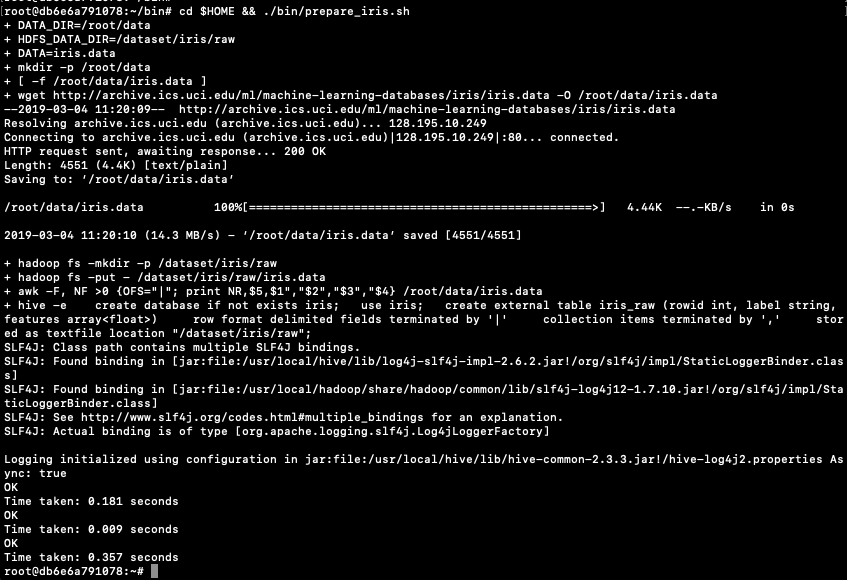
Using the IRIS data set as the data set (and loaded in previous post), the first thing we need to find is the minimum and maximum values for each feature.

select min(features[0]), max(features[0]),
       min(features[1]), max(features[1]),
       min(features[2]), max(features[2]),
       min(features[3]), max(features[3])
from iris_raw;

we get the following results.

4.3  7.9  2.0  4.4  1.0  6.9  0.1  2.5
 
The format of the results can be a little confusing. What this list gives us is the results for each of the four features. For feature[0], sepal_length, we have a minimum value of 4.3 and a maximum value of 7.9. Similarly, feature[1], sepal_width, min=2.0, max=4.4 feature[2], petal_length, min=1.0, max=6.9 feature[3], petal_width, min=0.1, max=2.5 To use these minimum and maximum values, we need to declare some local session variables to store these.

set hivevar:feature0_min=4.3;
set hivevar:feature0_max=7.9;
set hivevar:feature1_min=2.0;
set hivevar:feature1_max=4.4;
set hivevar:feature2_min=1.0;
set hivevar:feature2_max=6.9;
set hivevar:feature3_min=0.1;
set hivevar:feature3_max=2.5;

After setting those variables we can now write a SQL SELECT and use the add_bias function to perform the calculations.

select rowid, label,
       add_bias(array(
          concat("1:", rescale(features[0],${f0_min},${f0_max})), 
          concat("2:", rescale(features[1],${f1_min},${f1_max})), 
          concat("3:", rescale(features[2],${f2_min},${f2_max})), 
          concat("4:", rescale(features[3],${f3_min},${f3_max})))) as features
from iris_raw;

and we get

> 1 Iris-setosa   ["1:0.22222215","2:0.625","3:0.0677966","4:0.041666664","0:1.0"]
> 2 Iris-setosa   ["1:0.16666664","2:0.41666666","3:0.0677966","4:0.041666664","0:1.0"]
> 3 Iris-setosa   ["1:0.11111101","2:0.5","3:0.05084745","4:0.041666664","0:1.0"]
...

Other feature scaling methods, available in Hivemall, include L1/L2 Normalization and zscore.

Wednesday, March 13, 2019

OCI - Making DBaaS Accessible using port 1521

When setting up a Database on Oracle Cloud Infrastructure (OCI) for the first time there are a few pre and post steps to complete before you can access the database using a JDBC type of connect, just like what you have in SQL Developer, or using Python or other similar tools and/or languages.  

1. Setup Virtual Cloud Network (VCN)
The first step, when starting off with OCI, is to create a Virtual Cloud Network.

 Screenshot 2019-03-13 11.08.48


Create a VCN and take all the defaults. But change the radio button shown in the following image.
 Screenshot 2019-03-13 11.13.07

That's it. We will come back to this later.

2. Create the Oracle Database To create the database
select 'Bare Metal, VM and Exadata' from the menu.

 Screenshot 2019-03-13 11.14.08

Click on the 'Launch DB System' button.
 Screenshot 2019-03-13 11.15.28

 Fill in the details of the Database you want to create and select from the various options from the drop-downs.
 Screenshot 2019-03-13 11.16.56
Fill in the details of the VCN you created in the previous set, and give the name of the DB and the Admin password.
 Screenshot 2019-03-13 11.19.00
When you are finished everything that is needed, the 'Launch DB System' at the bottom of the page will be enabled. After clicking on this botton, the VM will be built and should be ready in a few minutes. When finished you should see something like this.
 Screenshot 2019-03-13 11.22.51  3. SSH to the Database server
 When the DB VM has been created you can now SSH to it. You will need to use the SSH key file used when creating the DB VM. You will need to connect to the opc (operating system user), and from there sudo to the oracle user. For example
 
<ssh file> opc@<public IP address>

The public IP address can be found with the Database VM details
 
Screenshot 2019-03-13 11.26.35
[opc@tudublins1 ~]$ sudo su - oracle
[oracle@tudublins1 ~]$ . oraenv
ORACLE_SID = [cdb1] ? 
The Oracle base has been set to /u01/app/oracle
[oracle@tudublins1 ~]$ 
[oracle@tudublins1 ~]$ sqlplus / as sysdba

SQL*Plus: Release 18.0.0.0.0 - Production on Wed Mar 13 11:28:05 2019
Version 18.3.0.0.0

Copyright (c) 1982, 2018, Oracle. All rights reserved.


Connected to:
Oracle Database 18c Enterprise Edition Release 18.0.0.0.0 - Production
Version 18.3.0.0.0

SQL> alter session set container = pdb1;

Session altered.

SQL> create user demo_user identified by DEMO_user123##;

User created.

SQL> grant create session to demo_user;

Grant succeeded.

SQL>

4. Open port 1521 
To be able to access this with a Basic connection in SQL Developer and most programming languages, we will need to open port 1521 to allow these tools and languages to connect to the database. To do this go back to the Virtual Cloud Networks section from the menu.

Screenshot 2019-03-13 11.08.48

Click into your VCN, that you created earlier. You should see something like the following.

Screenshot 2019-03-13 11.34.53

Click on the Security Lists, menu option on the left hand side.

Screenshot 2019-03-13 11.39.10
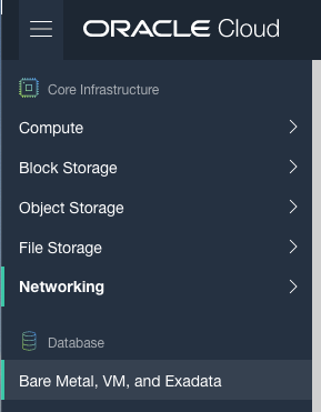
From that screen, click on Default Security List, and then click on the 'Edit All Rules' button at the top of the next screen. Add a new rule to have a 'Destination Port Range' set for 1521

Screenshot 2019-03-13 11.41.19

That's it.

 5. Connect to the Database from anywhere

Now you can connect to the OCI Database using a basic SQL Developer Connection.


Screenshot 2019-03-13 11.46.06

Wednesday, March 6, 2019

Moving Average in SQL (and beyond)

A very common analytics technique for financial and other data is to calculate the moving average. This can allow you to see a different type of pattern in your data that may not is evident from examining the original data.

But how can we calculate the moving average in SQL?

Well, there isn't a function to do it, but we can use the windowing feature of analytical SQL to do so. The following example was created in an Oracle Database but the same SQL (more or less) will work with most other SQL databases.
 
SELECT month, 
       SUM(amount) AS month_amount,
       AVG(SUM(amount)) OVER
          (ORDER BY month ROWS BETWEEN 3 PRECEDING AND CURRENT ROW) AS moving_average
FROM  sales
GROUP BY month
ORDER BY month;

This gives us the following with the moving average calculated based on the current value and the three preceding values, if they exist.
 
 MONTH MONTH_AMOUNT MOVING_AVERAGE
---------- ------------ --------------
         1     58704.52       58704.52
         2      28289.3       43496.91
         3     20167.83       35720.55
         4      50082.9     39311.1375
         5     17212.66     28938.1725
         6     31128.92     29648.0775
         7     78299.47     44180.9875
         8     42869.64     42377.6725
         9     35299.22     46899.3125
        10     43028.38     49874.1775
        11     26053.46      36812.675
        12     20067.28      31112.085

In some analytic languages and databases, they have included a moving average function. For example using HiveMall on Hive we have.
 
SELECT moving_avg(x, 3) FROM (SELECT explode(array(1.0,2.0,3.0,4.0,5.0,6.0,7.0)) as x) series;

If you are using Python, there is an inbuilt function in Pandas.
 
rolmean4 = timeseries.rolling(window = 4).mean()

Monday, March 4, 2019

HiveMall: Docker image setup

In a previous blog post I introduced HiveMall as a SQL based machine learning language available for Hadoop and integrated with Hive. If you have your own Hadoop/Big Data environment, I provided the installation instructions for Hivemall, in that blog post An alternative is to use Docker. There is a HiveMall Docker image available. A little warning before using this image. It isn't updated with the latest release but seems to get updated twice a year. Although you may not be running the latest version of HiveMall, you will have a working environment that will have almost all the functionality, bar a few minor new features and bug fixes. To get started, you need to make sure you have Docker running on your machine and you have logged into your account. The docker image is available from Docker Hub. Take note of the version number for the latest version of the docker image. In this example it is 20180924 
Screenshot 2019-03-04 10.53.57 
Open a terminal window and run the following command. This will download and extract all the image files.
docker pull hivemall/latest:20180924
Screenshot 2019-03-04 10.51.34 
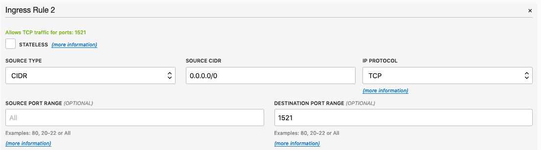
Until everything is completed. Screenshot 2019-03-04 11.01.40 
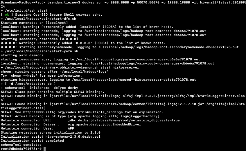
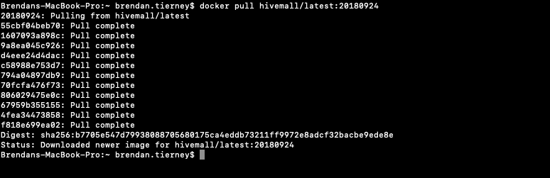
This docker image has HDFS, Yarn and MapReduce installed and running. This will require the exposing of the ports for these services 8088, 50070 and 19888. To start the HiveMall docker image run

docker run -p 8088:8088 -p 50070:50070 -p 19888:19888 -it hivemall/latest:20180924

Consider creating a shell script for this, to make it easier each time you want to run the image. Screenshot 2019-03-04 11.15.04
Now seed Hive with some data. The typical example uses the IRIS data set. Run the following command to do this. This script downloads the IRIS data set, creates a number directories and then creates an external table, in Hive, to point to the IRIS data set.
 
cd $HOME && ./bin/prepare_iris.sh
 

Screenshot 2019-03-04 11.20.49
Now open Hive and list the databases.

hive -S
hive> show databases;
OK
default
iris
Time taken: 0.131 seconds, Fetched: 2 row(s)

Connect to the IRIS database and list the tables within it.

hive> use iris;
hive> show tables;
iris_raw

Now query the data (150 records)

hive> select * from iris_raw;
1 Iris-setosa [5.1,3.5,1.4,0.2]
2 Iris-setosa [4.9,3.0,1.4,0.2]
3 Iris-setosa [4.7,3.2,1.3,0.2]
4 Iris-setosa [4.6,3.1,1.5,0.2]
5 Iris-setosa [5.0,3.6,1.4,0.2]
6 Iris-setosa [5.4,3.9,1.7,0.4]
7 Iris-setosa [4.6,3.4,1.4,0.3]
8 Iris-setosa [5.0,3.4,1.5,0.2]
9 Iris-setosa [4.4,2.9,1.4,0.2]
10 Iris-setosa [4.9,3.1,1.5,0.1]
11 Iris-setosa [5.4,3.7,1.5,0.2]
12 Iris-setosa [4.8,3.4,1.6,0.2]
13 Iris-setosa [4.8,3.0,1.4,0.1
...

Find the min and max values for each feature.

hive> select 
    > min(features[0]), max(features[0]),
    > min(features[1]), max(features[1]),
    > min(features[2]), max(features[2]),
    > min(features[3]), max(features[3])
    > from
    > iris_raw;

4.3  7.9  2.0  4.4  1.0  6.9  0.1  2.5

You are now up and running with HiveMall on Docker.