Showing posts with label ODM 11g R2. Show all posts

Friday, June 7, 2013

DBMS_PREDICTIVE_ANALYTICS & Predict

In this blog post I will look at the PREDICT procedure that is part of the DBMS_PREDICTIVE_ANALTYICS package. This package allows you to perform data mining in an automated way without having to go through the steps of building, testing and scoring data.

I had a previous blog post that showed how to use the EXPLAIN function to create an Attribute Importance model.

The predictive analytics procedures analyze and prepare the input data, create and test mining models using the input data, and then use the input data for scoring. The results of scoring are returned to the user. The models and supporting objects are not persisted and are removed from the database when the procedure is finished.

The PREDICT procedure should only be used for a Classification problem and data set.

The PREDICT procedure create a model based on the supplied data (out input table) and a target value,  and returns scored data set in a new table. When using PREDICT you do not get to select an algorithm to use.

The input data source should contain records that already have the target value populated.  It can also contain records where you do not have the target value. In this case the PREDICT function will use the records that have a target value to generate the model. This model will then score all records a the predicted target value

The syntax of the PREDICT procedure is:

DBMS_PREDICTIVE_ANALYTICS.PREDICT (
   accuracy OUT NUMBER,
   data_table_name IN VARCHAR2,
   case_id_column_name IN VARCHAR2,
   target_column_name IN VARCHAR2,
   result_table_name IN VARCHAR2,
   data_schema_name IN VARCHAR2 DEFAULT NULL);

Where

Parameter Name Description
accuracy This output parameter from the procedure. You do not pass anything into this parameter. The Accuracy value returned is the predictive confidence of the model generated/used by the PREDICT procedure
data_table_name The name of the table that contains the data you want to use
case_id_column_name The case id for each record. This is unique for each record/case.
target_column_name The name of the column that contains the target column to be predicted
result_table_name The name of the table that will contain the results. This table should not exist in your schema, otherwise an error will occur.
data_schema_name The name of the schema where the table containing the input data is located. This is probably in your current schema, so you can leave this parameter NULL.

The PREDICT procedure will produce an output tables (result_table_name parameter) and will contain 3 attributes.

CASE_ID This is the Case Id of the record from the original data_table_name. This will allow you to link up the data in the source table to the prediction in the result_table_name
PREDICTION This will be the predicted value of the target attribute
PROBABILITY This is the probability of the prediction being correct

Using the sample example data set that I have given in previous blog posts and in the blog post on the EXPLAIN procedure, the following code illustrates how to use the PREDICT procedure.

set serveroutput on

DECLARE
   v_accuracy NUMBER(10,9);
BEGIN
   DBMS_PREDICTIVE_ANALYTICS.PREDICT(
      accuracy => v_accuracy,
      data_table_name => 'mining_data_build_v',
      case_id_column_name => 'cust_id',
      target_column_name => 'affinity_card',
      result_table_name => 'PA_PREDICT');
   DBMS_OUTPUT.PUT_LINE('Accuracy of model = ' || v_accuracy);
END;

image

This took about 15 seconds to run on my laptop, which is surprisingly quick given all the work that is doing internally. To see the predictions and the results from the PREDICT procedure, you will need to query the PA_PREDICT table.

image

The final step that you might be interested in is to compare the original target value with the prediction value.

SELECT v.cust_id,
       v.affinity_card,
       p.prediction,
       p.probability
FROM   mining_data_build_v  v,
       pa_predict p
WHERE  v.cust_id = p.cust_id
AND    rownum <= 12;

image

Remember we do not get to see how or what Oracle did to generate these results. We do not get the opportunity to tune the process and the model.

So you have to be careful when you use the PREDICT function and on what data. Would you use this as a way to explore your data and to see if predictive analytics/data mining might be useful for your? Yes it would. Would you use it in a production scenario? the answer is maybe but it depends on the scenario. In reality if you want to do this in a production environment you will put some work into developing data mining models that best fit your data. To do this you will need to move onto the ODM tool and the DBMS_DATA_MINING package. But the PREDICT function is a quick way to get some small data scored (in some way) based on your existing data. If your marketing department says they want to start a tele marketing campaign in a couple of hours then PREDICT is what you need to use. It may not give you the most accurate of results, but it does give you results that you can start using quickly.

Tuesday, March 5, 2013

Clustering in Oracle Data Miner–Part 4

This is a the fourth part of a five (5) part blog post on building and using Clustering in Oracle Data Miner. The following outlines the contents of each post in this series on Clustering.
  1. The first part we looked at what clustering features exist in ODM and how to setup the data that we will be using in the examples
  2. The second part will focus on how to building Clusters in ODM .
  3. The third post will focus on examining the clusters produced by ODM and how to use the Clusters to apply to new data using ODM.
  4. The fourth post will look at how you can build and evaluate a Clustering model using the ODM SQL and PL/SQL functions.
  5. The fifth and final post will look at how you can apply your Clustering model to new data using the ODM SQL and PL/SQL functions.
With Clustering we are trying to find hidden patterns in our data. Unlike classification we a not directing the algorithms on what areas/attributes to focus on.
In my preceding post on Clustering in Oracle Data Miner I showed how you can use the Oracle Data Miner (ODM) tool, that is part of SQL Developer, to build a cluster model and to apply it to new data.
As I have shown in previous blog posts we can do all of the same steps using SQL and PL/SQL. In this blog post I will show you how to to these SQL and PL/SQL functions to generate a Clustering model and how you can evaluate the model produced.
Step 1 – What Cluster Models to we already have
Oracle Data Miner comes with a number of data dictionary tables. We can use these to see what already exists in our schema. In the example below we will have a look to see the Cluster models that were produced in the Part 2 blog post.
format model_name format a20
format mining_function format a20
format algorithm format a20

SELECT model_name,
       mining_function, 
       algorithm, 
       build_duration, 
       model_size
FROM ALL_MINING_MODELS
WHERE mining_function = 'CLUSTERING';

image
We can also look at the model settings that ODM produced. We can look at the settings of the K-Means model. This model (in my case) is called CLUS_KM_1_25.
column setting_value format a20
select setting_name,
         setting_value,
         setting_type
from  all_mining_model_settings
where model_name = 'CLUS_KM_1_25'

image
We can also look to see what attributes are used in the K-Mean model.
SELECT attribute_name, 
       attribute_type, 
       usage_type, 
       target
from  all_mining_model_attributes
where model_name = 'CLUS_KM_1_25'

image
I will show you how to use this Clustering model or the one that we are about to generate in my next blog post.
Step 2 – Creating the Setting table
When creating an Oracle Data Mining model in SQL you need to create Setting table. This will contain a record for each setting they you need to set for the algorithm you want to run. The settings table has a very basic structure and only consists of two columns. It is a good idea to create a separate Settings table for each algorithm or type of data mining you want to do. To create the settings table we run the following:
CREATE TABLE CLUSTER_SETTINGS (
Setting_Name  VARCHAR2(30),
Setting_Value VARCHAR2(4000));

The next step is to define the setting we want to use. The first of these will be the actual algorithm you want to run. Oracle has two Clustering algorithms: algo_kmeans and algo_o_cluster. In the examples we are working through we are using the K-Mean algorithm and we want to set the number of clusters to 10. We are also going to set the Automatic Data Preparation (ADP) on. Here is the code.
BEGIN
   INSERT INTO CLUSTER_SETTINGS (setting_name, setting_value)
   VALUES (dbms_data_mining.algo_name, dbms_data_mining.ALGO_KMEANS);
   INSERT INTO CLUSTER_SETTINGS (setting_name, setting_value)
   VALUES (dbms_data_mining.prep_auto, dbms_data_mining.PREP_AUTO_ON);
   INSERT INTO CLUSTER_SETTINGS (setting_name, setting_value)
   VALUES (dbms_data_mining.clus_num_clusters, 10);
  
   COMMIT;
END;

We can check to see that these records were inserted.
column setting_value format a25
select * from CLUSTER_SETTINGS;
image
The other settings will be dependent on what clustering algorithm is being used. Each one has their own setting. If you do not define any additional setting Oracle will use the in-build default settings.
To see what the default settings:
column setting_value format a35
select *
from table(dbms_data_mining.get_default_settings)
where setting_name like 'KM%';

image
If you want to use a different value to the default, just create a new record in the CLUSTER_SETTINGS table with the new value.

Step 3 – Create the new Cluster Model
We have the algorithm settings ready, so the next steps is to create the Cluster model. We will be using the DBMS_DATA_MINING.CREATE_MODEL function and pointing it to our CLUSTER_SETTINGS table.
BEGIN
   DBMS_DATA_MINING.CREATE_MODEL(
      model_name          => 'CLUSTER_KMEANS_MODEL',
      mining_function     => dbms_data_mining.clustering,
      data_table_name     => 'INSURANCE_CUST_LTV',
      case_id_column_name => 'CUSTOMER_ID',
      target_column_name  => null,
      settings_table_name => 'CLUSTER_SETTINGS');
END;

This takes a few seconds to run on my laptop. When finished we can uses queries like we used in Step 1 above to find out the details of what was produced.
Step 4 – Examining the Cluster model
The first thing that we will need to check is that the model was created.
format model_name format a20
format mining_function format a15
format algorithm format a15

SELECT model_name, 
       mining_function,
       algorithm,
       build_duration,
       model_size
FROM ALL_MINING_MODELS
WHERE mining_function = 'CLUSTERING';

image
One thing that is a bit curious is the mode size. We have basically created two K-means models using the same settings, but the final models have different sizes. See below for an explanation.
Now lets look at the algorithms settings for our new Cluster model (Cluster KMeans Model)
select setting_name,
       setting_value,
       setting_type
from  all_mining_model_settings
where model_name = 'CLUSTER_KMEANS_MODEL'

image
We can also look at the attributes used in the clusters.
SELECT attribute_name, 
       attribute_type, 
       usage_type, 
       target
from  all_mining_model_attributes
where model_name = 'CLUSTER_KMEANS_MODEL'
image
If we compare this list back to the list of attributes that were part of the model that we developed in the ODM tool, you will see that we have some extra attributes listed for the new K-means model.
The reason for these extra attributes and the bigger size (although still small) will be due to us having applied a sampling in the ODM tool. We took a subset of the data in the ODM tool and built the model based on this data. For the model we just created in SQL we took all the data (no sampling). That is why it would have looked at including more attributes because it was looking at a much bigger data set, etc.
Step 5 – Examining the Cluster Details
In this step we are going to look at some of the clusters produced by our new Cluster model.
We can produce the information relating to the clusters that were produced and what level in the hierarchy each cluster belongs. We can use this information to create/draw our own cluster hierarchy diagram.
set lines 90
column child format a40

select id, 
       record_count, 
       parent, 
       tree_level, 
       child
from table(dbms_data_mining.get_model_details_km('CLUSTER_KMEANS_MODEL'))

image
To look at the Centroid details for a particular cluster e.g. Cluster ID = 7, we can run:
column attribute_name format a25
column mode_value format a25

select t.id,
       c.attribute_name, 
       c.mean,
       c.mode_value,
       c.variance
from table (dbms_data_mining.get_model_details_KM('CLUSTER_KMEANS_MODEL')) t,
     table(t.centroid) c
where t.id = 7
order by c.attribute_name

The results will contain details of the centroid for cluster number 7. The centroid details will include the attributes that were used to form the centroid and the values for each attribute.
image
The last thing we can look at is the rule for a cluster. The following query will give you the full details of the cluster rule for Cluster 7. This will give for each attribute what the values or ranges of values that is used for that cluster. I’ll let you run this as it returns a large number of records. Run it and have a look at some of the output.
select t.id, 
       a.attribute_name, 
       a.conditional_operator,
       nvl(a.attribute_str_value,
       a.attribute_num_value) AS value,
       a.attribute_support,
       a.attribute_confidence
from TABLE(dbms_data_mining.get_model_details_km('CLUSTER_KMEANS_MODEL'))  t, 
     TABLE(t.rule.antecedent)  a
where t.id = 7
ORDER BY t.id, a.attribute_name, attribute_support, attribute_confidence desc, value;


My next blog post on Clustering in Oracle, will be the final one in the series. It will show you how to apply a Clustering model to new data in your database.

Wednesday, February 27, 2013

Clustering in Oracle Data Miner–Part 3

This is a the third part of a five (5) part blog post on building and using Clustering in Oracle Data Miner. The following outlines the contents of each post in this series on Clustering.

  1. The first part we looked at what clustering features exist in ODM and how to setup the data that we will be using in the examples
  2. The second part will focus on how to building Clusters in ODM .
  3. The third post will focus on examining the clusters produced by ODM and how to use the Clusters to apply to new data using ODM.
  4. The fourth post will look at how you can build and evaluate a Clustering model using the ODM SQL and PL/SQL functions.
  5. The fifth and final post will look at how you can apply your Clustering model to new data using the ODM SQL and PL/SQL functions.

In my previous posts on Clustering in ODM we have setup our data, we have explored it, we have taken a sample of the data and used this sample as input to the Cluster Build node. Oracle Data Miner has two clustering algorithms and our Cluster Build node created a clustering model for each.

In this post we will look at the next steps. The first of these is that we will look at examining what clustering models ODM produced. In the second part we will look at how we can use one of these clustering models to apply and label new data.

image

Step 1 – View the Cluster Models

To view the the cluster modes we need to right click the Cluster Build node and select View Models from the drop down list. We get an additional down down menu that gives the names of the two cluster models that were developed.

In my case these are called CLUS_KM_1_25 and CLUS_OC_1_25. You may get different numbers on your model names. These numbers are generated internally in ODM

image

The first mode that we will look at will be the K-Mean Cluster Model (CLUS_KM_1_25). Select this from the menu.

Step 2 – View the Cluster Rules

The hierarchical K-Mean cluster mode will be displayed. You might need to readjust/resize some of the worksheets/message panes etc in ODM to get the good portion of the diagram to display.

image

With ODM you cannot change, alter, merge, split, etc any the clusters that were generated. Oracle take the view of, this is what we have found it it up to you now to decide how you are going to use it.

To see that the cluster rules are for each cluster you can click on a cluster. When you do this you should get a pane (under the cluster diagram) that will contain two tabs, Centroid and Cluster Rule.

The Centroid tab provides a list of the attributes that best define the selected cluster, along with the average value for each attribute and some basic statistical information.

image

The Cluster Rules tab contains a set of rules that define the cluster in a IF/THEN statement format.

image

For each cluster in the tree we can see the number of cases in each cluster the percentage of overall cases for this cluster.

Work your way down the tree exploring each of the clusters produced.

The further down the tree you go the smaller the percentage of cases will fall into each cluster. In some tools you can merge these clusters. Not so in ODM. What you have to do is to use an IF statement in your code. Something like IF cluster_num IN (16, 17, 18, 19) THEN …..

Step 3 – Compare Clusters

In addition to the cluster tree, ODM also has two addition tabs to allow us to explore the clusters. These are Detail and Compare tabs.

image

Click on the Detail tab. We now get a detailed screen that contain various statistical information for each attribute. We can for each attribute get a histogram of the values within each attribute for this cluster.

We can use this important to start building up a picture of what each cluster might represent based on the values (and their distribution) for each cluster.

image

Try this out for a few clusters.

Step 4 – Multi-Cluster - Multi-variable Comparison of Clusters

The next level of comparison and evaluation of the clusters can be found under the Compare tab.

This lets us compare two clusters against each other at an attribute level. For example let us compare cluster 4 and 9. The attribute and graphics section gets updated to reflect the data for each of cluster. These are colour coded to distinguish the two clusters.

image 

We can work our way down through each attribute and again we can use this information to help us to understand what each cluster might represent.

An additional feature here is that we can do multi-variable (attribute) comparison. Holding down the control button select LTV_BIN, SEX and AGE. With each selection we get a new graph appearing at the bottom of the screen. This shows the distribution of the values by attribute for each cluster.  We can learn a lot from this.

image

So one possible conclusion we could draw from this data would be that Cluster 4 could be ‘Short Term Value Customers’ and Cluster 9 could be ‘Long Term Value Customer’

Step 5 – Renaming Clusters

When you have discovered a possible meaning for a Cluster, you can give it a meaningful name instead of it having a number. In our example, we would like to re-label Cluster 4 to ‘Short Term Value Customers’. To do this click on the Edit button that is beside the drop down that has cluster 4. Enter the new label and click OK.

SNAGHTML1bf2277

In the drop down we will now get the new label appearing instead of the cluster number.

Similarly we can do this for the other cluster e.g. ‘Long Term Value Customer’.

image


We have just looked at how to explore our K-Means model. You can do similar exploration of the O-Cluster model. I’ll leave that for you to do.


We have now explored our clusters and we have decided which of our Clustering Models best suits our needs. In our scenario we are going to select the K-Mean model to apply and label our new data.

Step 1 – Create the Apply Node

We have already setup our sample of data that we are going to use as our Apply Data Set. We did this when we setup the two different Sample node.

We are going to use the Sample node that was set to 40%.

The first step requires us to create an Apply Node. This can be found under the Component Palette and Evaluate and Apply tab. Click on the Apply node and move the mouse to the workflow worksheet and click near the Sample Apply node.

To connect the two nodes, move the mouse to the Sample Apply node and right click. Select Connect from the drop down menu and then move the mouse to the Apply node and click again. An connection arrow will be created joining these nodes.

Step 2 – Specify which Clustering Model to use & Output Data

Next we need to specify which of the clustering model we want to use to apply to our new data.

We need to connect the Cluster Build node to the Apply node. Move the mouse to the Cluster Build node, right click and select connect from the drop down menu. Move the mouse to the Apply node and click. We get the connection arrow between the two node.

We now have joined the Data and the Cluster Build node to the Apply node.

The final step is to specify what clustering mode we would like to use. In our scenario we are going to specify the K-Mean model.

(Single) Click the Cluster Build node. We now need to use the Property Inspector to select the K-Means model for the apply set. In the Models tab of the Property Inspector we should have our two cluster models listed. Under the Output column click in the box for the O-Cluster model. We should now get a little red X mark appearing. The K-Mean model should still have the green arrow under the Output column.

Step 3 – Run the Apply Node

We have one last data setup to do on the Apply node. We need to specify what data from the apply data set we want to include in the output from the Apply node.  For simplicity we want to just include the primary key, but you could include all the attributes.  In addition to including the attributes from the apply data source, the Apply Node will also create some attributes based on the Cluster model we selected. In our scenario, the K-Means model will create two additional attributes. One of these will contain the Cluster ID and the other attribute will be the probability of the that cluster being valid.

To include the attributes from the source data, double click on the Apply node. This will open the Edit Apply Node window. You will see that it already contains the two attributes that will be created by the K-Mean model.

image

To add the attributes from the source data, click on the Data Columns tab and then click on the green ‘+’ symbol. For simplicity we are going to just select the CUSTOMER_ID. Click the OK button to finish.

image

Now we are ready to run the Apply node. To do this right click on the Apply Node and select Run from the drop down menu. When everything is finished you will get the little green tick mark on the top right hand corner of the Apply node.

image

Step 4 – View the Results

To view the results and the output produced by the Apply node, right click on the Apply node and select View Data from the drop down menu.

We get a new tab opened in SQL Developer that will contain the data. This will consist of the CUSTOMER_ID, the K-means Cluster ID and the Cluster Probability. You will see that the some of the clusters assigned will have a number and some will have the cluster labels that we assigned in a previous step.

image

It is now up to you to decide how you are going to use this clustering information in an operational or strategic way in your organisation.


In my next (fourth) blog post in the series on Clustering in Oracle Data Miner, I will show how you can perform similar steps, of building and evaluating clustering models, using the SQL and PL/SQL functions in the database. So we will not be using the ODM tool. We will be doing everything in SQL and SQL/PLSQL.

Tuesday, February 19, 2013

Clustering in Oracle Data Miner–Part 2

This is a the second part of a five (5) part blog post on building and using Clustering in Oracle Data Miner. The following outlines the contents of each post in this series on Clustering.

  1. The first part we looked at what clustering features exist in ODM and how to setup the data that we will be using in the examples
  2. The second part will focus on how to building Clusters in ODM .
  3. The third post will focus on examining the clusters produced by ODM and how to use the Clusters to apply to new data using ODM.
  4. The fourth post will look at how you can build and evaluate a Clustering model using the ODM SQL and PL/SQL functions.
  5. The fifth and final post will look at how you can apply your Clustering model to new data using the ODM SQL and PL/SQL functions.

With Clustering we are trying to find hidden patterns in our data. Unlike classification we a not directing the algorithms on what areas/attributes to focus on.

In our scenario we want to look to see what distinct groupings or Segments that our Customer data naturally fit into. For each of these Segment Oracle Data Miner will tell us what attributes and the values of these attributes that determine if a customer belongs to one segment or another.

Step 1 - Define the Data Source

The first step involves us creating a Data Source Node for the table that we created and loaded in the previous blog post. We called this table INSURANCE_CUST_LTV.

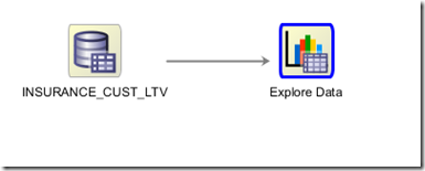
To create the Data Source Node go to the Component Palette. Under the Data tab you will find the Data Source option. Click on this and then go to the workflow worksheet and click. The Data Source node will be created and the wizard to specify the name of the table/view will open. Select INSURANCE_CUST_LTV from the list.

image

Click on the Next and then the Finish button to take in all the attribute.

Our data is now read to use.

Step 2 – Explore the Data

We can use the Explore Node to gather some statistics on the data and to produce some graphs.

To create the Explore Node, go to the Component Palette and under the Data tab you will find the Explore Data node. Click on this and then click again on the workflow worksheet, near the Data node.

You need to connect the Data node to the Explore Data node. Move your mouse to the Data node. Right-click this node and select Connect from the drop down menu. Then more the mouse to the Explore Data node and click on it. You will now have an arrowed line joining these two nodes

image

The next step we need to do is to right click on the Explore Data node and select Run from the drop down menu. ODM will go off to the database and gather various statistics and create a number of graphs based on the data in the table.

NB. If you click on the Explore Data node and then look in the Property Inspector you will see that ODM will take a sample of 2,000 records to produce the statistics and graphs. If you would like ODM to use all the records then you need to click the ‘Use All Data’ check box. Or you can change the sample size.

image

For your initial data investigation you might use the default of sampling 2,000 records before you increase the size of the sample.

In scenarios like this you may want to explore the data in more detail and to look at how the data is distributed in relation to certain attributes. In our data we have an attribute called LTV_BIN. In this attribute we have four values including, Very High, High, Medium and Low.

In our scenario, it might be more interesting to explore the data based on this attribute and it’s values. To do this we need to tell the Explore Data node to group the data analysis based on the values in this attribute.

image

Double-click the Explore Data node. In the Group By drop down select LTV_BIN. Click the OK button. You are now ready to run the Explore Data Node. To do this, right click on Explore Data node and select Run from the drop down list.

To view the statistics gathered and the graphs produced on the default sample of 2,000 records, right click the Explore Data node and select View Data from the drop down menu. You will get a new tab/window opening in SQL Developer with all the results.

image

This kind of data analysis only works with an attribute that has a low number of possible values.

Step 3 – Defining the data we will used to Build our Cluster models

We are going to divide the data in our CUST_INSURANCE_LTV into two data sets. The first data set will be used to build the Cluster models. The second data set will be used as part of the Apply node in my next blog post (part 3).

To divide the data we are going to use the Sample Node that can be found under the Transformation tab of the Component Palette.

Create your first Sample Node. In the Settings tab of the Property Inspector set the sample size to 60% and in the Details tab rename the node to Sample Build.

image

Create a second Sample node and give it a sample size of 40%. Rename this node to Sample Apply.

Right click on each of these Sample nodes to run them and have them ready for the next step of building the Clustering models.

image

Step 4 – Creating the Clustering Build Node

When you have finished exploring the data you are now ready to move on to creating the Clustering models. As ODM has two clustering algorithms, ODM will default to creating two Clustering models.

To create the Clustering models, go to the Component Palette. Under the Models tab, select Clustering.

image

Move the mouse to the workflow worksheet, near the Sample Build node and click the worksheet. The Clustering node will be created. Now we need to connect the data with the Clustering node. To do this right click on the Sample Build node and select Connect from the drop down list. Then move the mouse to the Clustering node and click. An arrowed line will be created connecting the two nodes.

image

At this point we can run the Clustering Build node or we can have a look at the setting for each algorithm.

Step 5 – The Clustering Algorithm settings

To setup the Cluster Build node you will need to double click on the node to open the properties window. The first thing that you need to do is to specify the Case ID (i.e. the primary key). In our example this is the CUSTOMER_ID.

SNAGHTML5b02a0

Oracle Data Miner has two clustering algorithms. The first of these is the well know k-Means (it is an enhanced version of it) and the O-Cluster. To look at the settings for each algorithm, click on the model listed under Model Settings and then click on the Advanced button.

A new window will open that lists all the attributes for the in the data source. The CUSTOMER_ID is unchecked as we said that this was the CASE_ID.

Click on the Algorithm Settings tab to see the internal settings for the k-means algorithm. All of these settings have a default value. Oracle has worked out what the optimal setting are for you. The main setting that you might want to play with is the Number of Clusters to build. The default is 10, but you might want to play with numbers between 5 and 15 depending on the number of clusters or segments you want to see in your data.

To view the algorithm settings for O-Cluster click on this under the Model Setting. We have less internal settings to worry about here, but we again can determine how many clusters we want to produce.

For our scenario we are going to take the default settings.

Step 6 – Run/Generate the Clustering models

At this stage we have the data set-up, the Cluster Build node created and the algorithm setting all set to what we want.

Now we are ready to run the Cluster Build node.

To do this, right click on the Cluster Build node and click run. ODM will go create a job that will contain PL/SQL code that will generate a cluster model based on K-Means and a second cluster model based on O-Cluster. This job will be submitted to the database and when it is completed we will get the little green tick mark on the top right hand corner of the Cluster Build node.

image


In the next blog post we will look at how to examine what clusters were produced by ODM and how we can take one of these and apply them to new data.

Wednesday, February 13, 2013

Clustering in ODM–Part 1

This is a the first part of a five (5) part blog post on building and using Clustering in Oracle Data Miner. The following outlines the contents of each post in this series on Clustering.

  1. This post part we will look at what clustering features exist in ODM and how to setup the data that we will be using in the examples
  2. The second part will focus on how to building Clusters and examining the clusters produced in ODM .
  3. The third post will focus on using the Clusters to apply to new data using ODM.
  4. The fourth post will look at how you can build and evaluate a Clustering model using the ODM SQL and PL/SQL functions.
  5. The fifth and final post will look at how you can apply your Clustering model to new data using the ODM SQL and PL/SQL functions.

Clustering is an unsupervised technique designed groupings of related data that are more similar to each other and are less similar to other groups.  Typically clustering is used in customer segmentation analysis to try an better understand what type of customers you have.

Like with all data mining techniques, Clustering will not tell you or give you some magic insight into your data. Instead it gives you more information for you to interpret and add the business meaning to them. With Clustering you can explore the data that forms each cluster to understand what it really means.

The Clusters give by Oracle Data Miner are just patterns that it has found in the data.

image

Oracle has two Clustering algorithms:

K-Means : Oracle Data Miner runs an enhanced version of the typical k-means algorithm. ODM builds models in a hierarchical manner, using a top-down approach with binary splits and refinements of all nodes at the end. The centroid of the inner nodes in the hierarchy are updated to reflect changes as the tree grows. The tree grows one node at a time. The node wit the largest variance is split to increase the size of the tree until the desired number of clusters is reached.

O-Cluster : O-Cluster is an Orthogonal Partitioning Clustering that creates a hierarchical grid based clustering model. It operates recursively, generating a hierarchical structure. The resulting clusters define dense areas.

The Data Set for out Clustering examples

I’m going to use a data set that is available on OTN (somewhere) and has been used for demos in the prior versions of ODM before the 11gR2 version (SQL Developer 3). It has gone by many names but the table name we care going to use is INSURANCE_CUST_LTV.

The file is in CSV format and we will use the Import feature in SQL Developer to import it.

1. In the schema you are using for Oracle Data Miner, right click Tables in the Connections tab. The Import option will appear on the menu. Select this.

image

2. Go to the directory where you saved the file, select it and then click on the Open button.

SNAGHTML60a28d3

3. You need to set the file Format to be ‘Delimited’ and the Delimiter set to ‘|’

SNAGHTML60c6d04

4. In the next step give the table name as INSURANCE_CUST_LTV

5.In the next step Select all the Attributes. It should default to this. Click next.

6. In Step 4 of the Wizard you can set the data types for each attribute. The simplest way is to set the character attributes to VARCHAR2 (50) :

CUSTOMER_ID,  LAST,  FIRST,  STATE,  REGION,  SEX,  PROFESSION,  BUY_INSURANCE (set this one to 3), MARITAL_STATUS, LTV_BIN

Set all the number attributes (all the others) to NUMBER without any precision or scale.

7. Click the next button and then the finish button.  SQL Developer will now load 15,342 records into the INSURANCE_CUST_LTV table, with no errors (hopefully!)


We are now ready to start our work with the Clustering algorithms in ODM.

In the next blog post we will look at exploring the data, building our Clustering models and examining the clusters that were produced by ODM.

Thursday, January 17, 2013

The ‘Oh No You Don’t’ of (Oracle) Data Science

Over the past couple of weeks I’ve had conversations with a large number of people about Data Science in the Oracle arena.

A few things have stood out. The first and perhaps the most important of these is that there is confusion of what Data Science actually means. Some think it is just another name for Statistics or Advanced Statistics, some Predictive Analytics or Data Mining, or Data Analysis, Data Architecture, etc.. The reality is it is not. It is more than what these terms mean and this is a topic for discussion for another day.

During these conversations the same questions or topics keep coming up and the simplest answer to all of these is taken from a Pantomime (Panto).

We need to have lots of statisticians
       'Oh No You Don't !'
We can only do Data Science if we have Big Data
        'Oh No You Don't !'
We can only do data mining/data science if we have 10’s or 100’s of Million of records
        'Oh No You Don't !'
We need to have an Exadata machine
        'Oh No You Don't !'
We need to have an Exalytics machine
        'Oh No You Don't !'
We need extra servers to process the data
        'Oh No You Don't !'
We need to buy lots of Statistical and Predictive Analytics software
        'Oh No You Don't !'
We need to spend weeks statistically analysing a predictive model
        'Oh No You Don't !'
We need to have unstructured data to do Data Science
        'Oh No You Don't !'
Data Science is only for large companies
        'Oh No You Don't !'
Data Science is very complex, I can not do it
        'Oh No You Don't !'

Let us all say it together for one last time ‘Oh No You Don’t

In its simplest form, performing Data Science using the Oracle stack, just involves learning and using some simple SQL and PL/SQL functions in the database.

Maybe we (in the Oracle Data Science world and those looking to get into it) need to adopt a phrase that is used by Barrack Obama of ‘Yes We Can’, or as he said it in Irish when he visited Ireland back in 2011, ‘Is Feidir Linn’.

Remember it is just SQL.

Wednesday, January 2, 2013

OUG Norway April 2013 - New Year’s News

I received an email at 23:24 on the 1st January from the OUG in Norway telling me that I’ve had two presentations accepted for the Annual OUG Norway seminar event. This will be on during the 17th-19th April.

The first day of this event (17th April) will be held in a hotel in Oslo. Then on the morning of 18th April we board the Color Magic cruise for the next two days of the conference. The ferry/cruise will go from Oslo to Kiel in Germany and then back again to Oslo, returning around 10am on Saturday 20th April.

I will be giving two presentations on the Oracle Advanced Analytics Option. The first presentation, ‘Using Predictive Analytics in Oracle’, will give an overview of the Oracle Advanced Analytics Option and will then focus on the Oracle Data Miner work-flow tool. This will presentation will include a live demo of using Oracle Data Miner to create some data mining models.

The second presentation, ‘How to Deploy and Use your Oracle Data Miner Models in Production’, builds on the examples given in the first presentation and will show how you can migrate, user and update your Oracle Data Miner models using the features available in SQL and PL/SQL. Again a demo will be given.

Wednesday, December 19, 2012

Association Rules in ODM-Part 4

This is a the final part of a four part blog post on building and using Association Rules in the Oracle Database using Oracle Data Miner. The following outlines the contents of each post in the series on Association Rules

  1. This first part will focus on how to building an Association Rule model
  2. The second post will be on examining the Association Rules produced by ODM – This blog post
  3. The third post will focus on using the Association Rules on your data.
  4. The final post will look at how you can do some of the above steps using the ODM SQL and PL/SQL functions.

In my previous posts I showed how you can go about setting up for Association Rule analysis in Oracle Data Miner and how to examine the rules that are generated.

This post will focus on how we build and use association rules using the functionality that is available in SQL and PL/SQL.

Step 1 – Build the Settings Table

As with all Oracle Data Mining functions in SQL and PL/SQL you will need to setup or build a settings table. This table contains all the settings necessary to run the model build functions. It is a good idea to create a separate settings table for each model build that you complete.

CREATE TABLE assoc_sample_settings (
setting_name VARCHAR2(30),
setting_value VARCHAR2(4000));

Step 2 – Define the Settings for the Model

Before you go to generate your model you need to set some of the parameters for the algorithm. To start with you need to defined that we are going to generate an Association Rules model, turn off the Automatic Data Preparation.

We can also set 3 additional settings for Association Rules.


image


The ASSO_MIN_SUPPORT has a default of 0.1 or 10%. That means that only rules that exist in 10% or more of the cases will be generated. This is really a figure that is too high. In the code below we will set this to a 1%. This matches the settings that we used in SQL Developer in my previous posts.


BEGIN


INSERT INTO assoc_sample_settings (setting_name, setting_value) VALUES

(dbms_data_mining.algo_name, dbms_data_mining.ALGO_APRIORI_ASSOCIATION_RULES);


INSERT into assoc_sample_settings (setting_name, setting_value) VALUES

(dbms_data_mining.prep_auto, dbms_data_mining.prep_auto_off);


INSERT into assoc_sample_settings (setting_name, setting_value) VALUES

(dbms_data_mining.ODMS_ITEM_ID_COLUMN_NAME, ‘PROD_ID’);


INSERT into assoc_sample_settings (setting_name, setting_value) VALUES

(dbms_data_mining.ASSO_MIN_SUPPORT, 0.01);


COMMIT;


END;

/


Step 3 – Prepare the Data


In our example scenario we are using the SALE data that is part of the SH schema. The CREATE_MODEL function needs to have an attribute (CASE_ID) that identifies the key of the shopping basket. In our case we have two attributes, so we will need to use a combined key. This combined key consists of the CUST_ID and the TIME_ID. This links all the transaction records related to the one shopping event together.


We also just need the attribute that has the information that we need. In our Association Rules (Market Basket Analysis) scenario, we will need to include the PROD_ID attribute. This contains the product key of each product that was included in the basket


CREATE VIEW ASSOC_DATA_V AS (

SELECT RANK() OVER (ORDER BY CUST_ID, TIME_ID) CASE_ID,


t.PROD_ID


FROM SH.SALES t );


Step 4 – Create the Model


We will need to use the DBMS_DATA_MINING.CREATE_MODEL function. This will use the settings in our ASSOC_SAMPLE_SETTINGS table. We will use the view created in Step 3 above and use the CASE_ID attribute we created as the Case ID in the function all.


BEGIN 
   DBMS_DATA_MINING.CREATE_MODEL( 
     model_name          => 'ASSOC_MODEL_2', 
     mining_function     => DBMS_DATA_MINING.ASSOCIATION, 
     data_table_name     => 'ASSOC_DATA_V', 
     case_id_column_name => ‘CASE_ID’, 
     target_column_name  => null, 
     settings_table_name => 'assoc_sample_settings');


END;


On my laptop this took approximately 5 second to run on just over 918K records involving just over 143K cases or baskets.


Now that is quick!!!


Step 5 – View the Model Outputs


There are a couple of functions that can be used to extract the rules produced in our previous step. These include:


GET_ASSOCIATION_RULES : This returns the rules from an association model.


SELECT rule_id, 
       antecedent, 
       consequent, 
       rule_support,


       rule_confidence


FROM TABLE(DBMS_DATA_MINING.GET_ASSOCIATION_RULES('assoc_model_2', 10));


The 10 here returns the top 10 records or rules.image GET_FREQUENT_ITEMSETS : returns a set of rows that represent the frequent item sets from an association model. In the following code we want the top 30 item sets to be returned, but filtered to only display item sets where there are 2 or more rules.


SELECT itemset_id,

       items,


       support,


       number_of_items


FROM TABLE(DBMS_DATA_MINING.GET_FREQUENT_ITEMSETS('assoc_model_2', 30))


WHERE number_of_items >= 2;


image

Thursday, November 29, 2012

Association Rules in ODM-Part 3

This is a the third part of a four part blog post on building and using Association Rules in Oracle Data Miner. The following outlines the contents of each post in the series on Association Rules

  1. This first part will focus on how to building an Association Rule model
  2. The second post will be on examining the Association Rules produced by ODM – This blog post
  3. The third post will focus on using the Association Rules on your data.
  4. The final post will look at how you can do some of the above steps using the ODM SQL and PL/SQL functions.

In my previous posts I showed how you can go about setting up for Association Rule analysis in Oracle Data Miner and how to examine the rules that are generated.

This post will focus on how we can extract and use these rules in Oracle Data Miner.

Step 1 – Model Details

Association Rules are an unsupervised method of data mining. In Oracle Data Miner we cannot use the Apply node to to score new data. What we have to do is to generate the Model Details. These in turn can then be used.

The Model Details node is used when we do unsupervised learning to extract the rules that are generated.

To do this we need to click on the Model Details node in the Models section of the Component Palette and then click on our workspace, just to the right of the Association Rule node.

The Edit Model Selection window will open. Connect the Association Rule node to the Model Details node. Then Run the node. This will then generate the Association Rules in a format what we can reuse.

image

When you get the small green tick on the Model Details node you can then view what was generated.

Right click on the Model Details node and click on View Details from the menu.

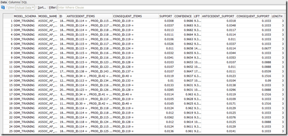
image

The output is similar to what we would have seen under the Association Rule node with the addition of a few more attributes that include the schema name and model name.

We can order the rules based on the Confidence level by double clicking on the Confidence column header. You might need to do this twice to get the rule appearing based on a descending confidence value.

At this point we can no look at persisting the Association Rules. See step 2 below.

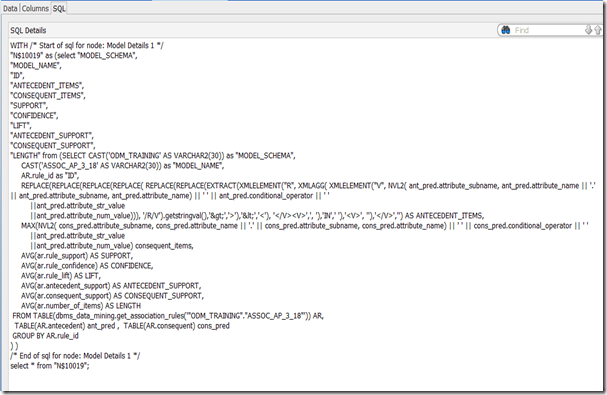
We can also view the SQL that was used to generate the Association Rules that we see in the Model Details node. While still viewing the rules, click on the SQL tab.

image

Step 2 – Persisting the Association Rules

To make the rules persist and be useable outside of ODM we can persist the Association Rules in a table. The first step to do this is to create a new Table Node. This can be found under the Data section of the Component Palette. Click this Create Table or View node in the component palette and then click on the workspace, just to the right of the Model Details node.

Connect the Model Details node to the Output node, by right clicking on the Model Details node, select Connect from the menu and then click on the Output Node.

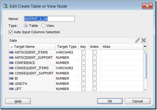
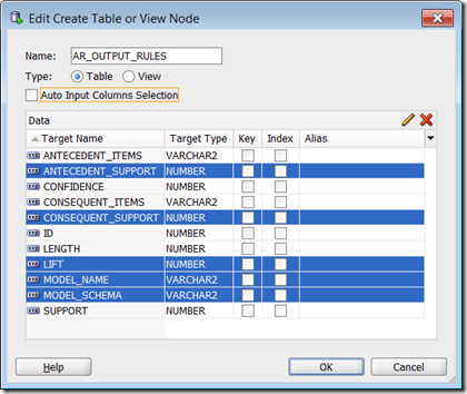
We can now edit the format of the Output i.e. specify what attributes are to be in our Output table. Double click on the Output node or right click and select Edit from the menu. We now get the Edit Create Table or View Node.

SNAGHTML18801036

We can give the output a meaningful name e.g. AR_OUTPUT_RULES. We can also specify what rule properties we can to export to attributes in out table.

We will need to un-tick the Auto Input Columns Selection tick box before we can remove any of the output attributes. In my case I only want to have ANTECENDENT_ITEMS, CONSEQUENT_ITEMS, ID, LENGTH, CONFIDENCE and SUPPORT in my out put. So I need to select and highlight all the other attributes (holding the control button). After selecting all the attributes I do not want included in the final output table, I need to click on the red X icon.

SNAGHTML18859128

When complete click on the OK button to go back to the workflow.

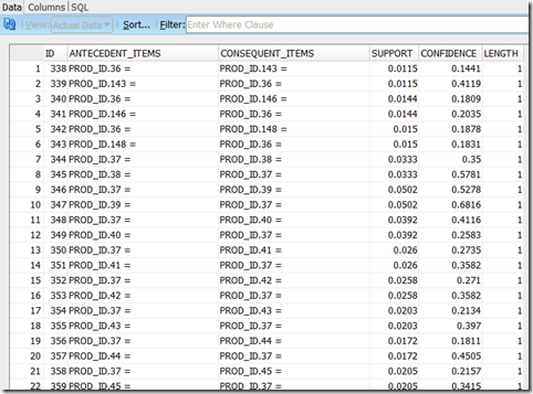
To generate the table right click on the AR_OUTPUT_RULES node and select Run from the menu. When you get the green tick mark on the AR_OUTPUT_RULES node the table has been created with records containing the details of each rules.

image

To view the contents of the AR_OUTPUT_RULES table we can right click on this node and select view data from the menu.

image

We can now use these rules in our applications.


Check out the next post in the series (Part 4) where we will look at the functionality available in the ODM SQL & PL/SQL functions to perform Association Rule analysis.