Showing posts with label ODM 11g R2. Show all posts

Tuesday, November 27, 2012

Association Rules in ODM–Part 2

This is a the second part of a four part blog post on building and using Association Rules in Oracle Data Miner.  The following outlines the contents of each post in the series on Association Rules

  1. This first part will focus on how to building an Association Rule model
  2. The second post will be on examining the Association Rules produced by ODM – This blog post
  3. The third post will focus on using the Association Rules on your data.
  4. The final post will look at how you can do some of the above steps using the ODM SQL and PL/SQL functions. 

In the previous post I looked at the steps needed to setup a data source and to setup the Association Rule node. When everything was setup we ran the workflow.

Step 1 – Viewing the Model

We the workflow has finished running we will have the green tick marks on each node. This is where we left thing at the end of the previous post (Part 1). To view the model details, right click on the Association Role Node and select View Models from the menu.

image

There are 3 main concepts that are important in relation to Association Rules:

  • Support: is the proportion of transactions in the data set that contain the item set i.e. the number of times the rule occurs
  • Confidence: is the proportion of the occurrences of the antecedent that result in the consequent e.g. how many times do we get C when we have A and B  {A, B} => C
  • Lift: indicates the strength of a rule over the random co-occurrence of the antecedent and the consequent

Support and Confidence are the primary measures that are used to access the usefulness of an association rule.

In our example we can see that the the antecedent and the consequent has numbers separated by the word AND. These numbers correspond to the product numbers.

Step 2 – Examining the Model Rules

To read the antecedent and the consequent for the first rule in our example we have:

Antecedent: 137 AND 143 AND 128

Consequent: 144

To read this association rule we would say that if a Customer bought product 137 and product 143 and product 128, then we have a Confidence value of almost 71%. This is a strong association.

We can check the ordering of the rules by changing the Sort By criteria. As Confidence and Support are the main ways to evaluate the rules, we can change the Sort By criteria to be Confidence. Then click on the Query button to refresh the rules section.

image

Here get a list of the strongest rules listed in descending order.

Below the section of the screen that has the Rules, we have the Rule Details section.

image 

Here we can see that the rule gets formatted into an IF statement. The first rule in the list has a confidence of almost 97%. As it is a simple IF statement it can be easily implemented in our applications.

We want use the information that these rules provides in a number of ways. One such consequence of these rules is that we can look at improving the ordering and distribution of these products to ensure that we have sufficient numbers of each. Another consequence is that we can enhance the front end selling mechanism to make sure that if a customer is buying product 114, 118 and 115 then we can remind the customer of product 119. We can also ensure that all these products are not located beside each other, so that the customer will have to walk past many other products in order to find them. That is why we never see milk and bread beside each other in a grocery store.

Step 3 – Applying Filters to the Model Rules

In the previous step we were able to sort our rules based on some of the measures of our Association Rules and to see how these rules are structured.

Association Rule Analysis can generate many thousands of possible rules for a small data set. In some cases the similar rules can appear and we can have lots of rules that occur so infrequently that they are perhaps meaningless.

ODM provides us with a number of filters that we can apply to the rules that enables use to look for the rules that are of must interest to use. We can access these filters by clicking on the More button, that is located just under the Query button.

We can refine our query on the rules based on the various measures and the number if items in the rule. In addition to this we can also filter based on the values of the items. This is particularly useful if we want to concentrate on specific items (in our example Products). To illustrate this use focus on the rules that involve Product 115. Click on the green + symbol on the right hand side of the window. Select 115 from the list provided. Next we need to decide if we want Product 115 involved in the Antecedent or the Consequent. In our example select the Consequent. This is located to the bottom right of the window. Then click the OK button and then click on the Query button to update the list of rules that correspond with the new filter.

image

We can see that we only have rules that have Product 115 in the Consequent column.

We can also see that we have 134 rules for this scenarios out of a total of 20,988 (your results might differ slightly to mine and that’s OK. It really depends on what version of the sample data you are using)


Check out the next post in the series (Part 3) where we will look at how you can use the Association Rules produced by ODM.

Friday, November 23, 2012

Association Rules in ODM–Part 1

This is a the first part of a four part blog post on building and using Association Rules in Oracle Data Miner. The following outlines the contents of each post in the series on Association Rules

  1. This first part will focus on how to building an Association Rule model
  2. The second post will be on examining the Association Rules produced by ODM – This blog post
  3. The third post will focus on using the Association Rules on your data.
  4. The final post will look at how you can do some of the above steps using the ODM SQL and PL/SQL functions.

image

The data set we will be using for Association Rule Analysis will be the sample data that comes with the SH schema in the database. Access to this schema and it’s data was setup when we created our data mining schema and ODM Repository.

Step 1 – Getting setup

As with all data mining projects you will need a workspace that will contain your workflows. Based on my previous ODM blog posts you will have already created a Project and some workflows. You can either reuse an existing workflow you have used for one of the other ODM modeling algorithms or you can create a new Workflow called Association Rules.

Step 2 – Define your Data Set

Assuming that your database has been setup to have the Sample schemas and their corresponding data, we will be using the data that is in the SH schema. In a previous post, I gave some instructions on setting up your database to use ODM and part of that involved a step to give your ODM schema access to the sample schema data.

We will start off by creating a Data Source Node. Click on the Data Source Node under the Component Palette. Then move your mouse to your your workspace area and click. A Data Source Node will be created and a window will open. Scroll down the list of Available Tables until you find the SH.SALES table. Click on this table and then click on the Next button. We want to include all the data so we can now click the Finish Button.

image

Our Data Source Node will now be renamed to SALES.

Step 3 – Setup the Association Build Node

Under the Model section of the Component Palette select Association. Move the mouse to your work area (and perhaps just the to right of the SALES node) click. Our Association Node will be created.

image

For the next step we need to join the our data source (SALES) with the Association Build Node. Right click on the SALES data node and select Connect from the drop down menu. Then move the mouse to the Association Build node and click. You should now have the two nodes connected.

We will now get the Edit Association Build Node property window opening for us. We will need to enter the following information:

  • Transaction ID: This is the attribute(s) that can be used to uniquely identify each transaction. In our example the Customer ID and the Time ID of the transaction allows us to identify what we want to analyse by i.e. the basket. This will group all the related transactions together
  • Item ID: What is the attribute of the thing you want to analyse. In our case we want to analyse the Products purchased, so select PROD_ID in this case
  • Value: This is an identifier used to specify another column with the transaction data to combine with the Item ID. <Existence> means that you want to see if there are any type of common bundling among all values of the selected Item ID. Use this.

image

Like all data mining products, Oracle has just one Algorithm to use for Association Rule Analysis, the Apriori Algorithm.

Click the OK button. You are now ready to run the Association Build Node. Right click on the node and select Run from the menu. After a short time everything should finish and we will have the little green tick makes on each of the nodes.

image


Check out the next post in the series (Part 2) where we will look at how you can examine the rules produced by our model in ODM.

Friday, November 16, 2012

Accepted for BIWA Summit–9th to 10th January

I received an email today to say that I had a presentation accepted for the BIWA Summit. This conference will be in the Sofitel Hotel beside the Oracle HQ in Redwood City.

The title of the presentation is “The Oracle Data Scientist” and the abstract is

Over the past 18 months we have seen a significant increase in the demand for Data Scientists. But how does someone become a data scientist. If we examine the requirements and job descriptions of this role we can see that being able to understand and process data are fundamental skills. So an Oracle developer is ideally suited to being a Data Scientist. The presentation will show how an  Oracle developer can evolve into a data scientist through a number of stages, including BI developer, OBIEE developer, statistical analysis, data miner and data scientist. The tasks and tools will be discussed and explored through each of these roles. The second half of the presentation will focus on the data mining functionality available in SQL and PL/SQL. This will consist of a demonstration of an Analytics Development environment and how you can migrate (and use) your models in a Production environment

For some reason Simon Cowell of XFactor fame kept on popping into my head and it now looks like he will be making an appearance in the presentation too. You will have to wait until the conference to find out what Simon Cowell and Being an Oracle Data Scientist have in common.

Check out the BIWA Summit website for more details and to register for the event.

I’ll see you there Smile

Saturday, October 20, 2012

Oracle Advanced Analytics Option in Oracle 12c

At Oracle Open World a few weeks ago there was a large number of presentations on Big Data and Analytics.  Most of these were marketing type presentations, with a couple of presentations on using R and how it can not be integrated into the Oracle Database 11.2.

In addition this these there was one presentation that focused on the Oracle Advanced Analytics (OAA) Option.

The Oracle Advanced Analytics Option covers the Oracle Data Mining features and the Oracle R Enterprise features in the Database.

The purpose of this blog post is to outline and summarise what was mentioned at these presentations, and will include what changes are/may be coming in the “Next Release” of the database i.e. Oracle 12c.

Health Warning: As with all the presentations at OOW that talked about what may be in or may be in the next release, there is not guarantee that the features will actually be in the release version of the database. Here is the slide that gives the Safe Harbor statement.

image

  • 12c will come with R embedded into it. So there will be no need for any configurations.
  • Oracle R client will come as part of the server install.
  • Oracle R client will be able to use the Analytics functions that exist in the database.
  • Will be able to run R code in the database.
  • The database (12c) will be able to spawn multiple R engines.
  • Will be able to emulate map-reduce style algorithms.
  • There will be new PREDICTION function, replacing the existing (11g) functionality. This will combine a number of steps of building a model and applying it to the data to be scored into one function.  But we will still need the functionality of the existing PREDICTION function that is in 11g. So it will be interesting to see how this functionality will be kept in addition to the new functionality being proposed in 12c.
  • Although the Oracle Data Miner tool will still exits and will have many new features. It was also referred to as the ‘OAA Workflow’.  So those this indicate a potential name change?  We will have to wait and see.
  • Oracle Data Miner will come with a new additional graphing feature. This will be in addition to the Explore Node and will allow us to produce more typical attribute related graphs. From what I could see these would be similar to the type of box plot, scatter, bar chart, etc. graphs that you can get from R.
  • There will be a number of new algorithms too, including a useful One Class Support Vector Machine. This can be used when we have a data set with just one class value. This algorithm will work out what records/cases are more important and others.
  • There will be a new SQL node. This will allow us to write our own data transformation code.
  • There will be a new node to allow the calling of R code.
  • The tool also comes with a slightly modified layout and colour scheme.

Again, the points that I have given above are just my observations. They may or may not appear in 12c, or maybe I misunderstood what was being said.

It certainly looks like we will have a integrate analytics environment in 12c with full integration of R and the ODM in-database features.

Wednesday, October 17, 2012

Extracting the rules from an ODM Decision Tree model

One of the most interesting of important aspects of a Decision Model is that we as a user can get to see what rules the machine learning algorithm has generated for our data.

I’ve give a number of examples in various blog posts over the past few years on how to generate a number of classification models. An example of the workflow is below.

SNAGHTML207172c9

In the Class Build node we get four models being generated. These include a Generalised Linear Model, Support Vector Machine, Naive Bayes and a Decision Tree model.

We can explore the Decision Tree model by right clicking on the Class Build Node, selecting View Models and then the Decision Tree model, which will be labelled with a ‘DT’ in the name.

image

As we explore the nodes and branches of the Decision Tree we can see the rule that was generated for a node in the lower pane of the applications. So by clicking on each node we get a different rule appearing in this pane

image

Sometimes there is a need to extract this rules so that they can be presented to a number of different types of users, to explain to them what is going on.

How can we extract the Decision Tree rules?

To do this, you will need to complete the following steps:

  • From the Models section of the Component Palette select the Model Details node.
  • Click on the Workflow pane and the Model Details node will be created
  • Connect the Class Build node to the Model Details node. To do this right click on the Class Build node and select Connect. Then move the mouse to the Model Details node and click. The two nodes should now be connected.
  • Edit the Model Details node, uncheck the Auto Settings, select Model Type to be Decision Tree, Output to be Full Tree and all the columns.

SNAGHTML2093297b

  • Run the Model Details node. Right click on the node and select run. When complete you you will have the little green box with a tick mark, on the top right hand corner.
  • To view the details produced, right click on the Model Details node and select View Data
  • The rules for each node will now be displayed. You will need to scroll to the right of this pane to get to the rules and you will need to expand the columns for the rules to see the full details

image

Friday, October 12, 2012

My Presentations on Oracle Advanced Analytics Option

I’ve recently compiled my list of presentation on the Oracle Analytics Option. All these presentations are for a 45 minute period.

I have two versions of the presentation ‘How to do Data Mining in SQL & PL/SQL’, one is for 45 minutes and the second version is for 2 hour.

I have given most of these presentations at conferences or SIGS.

Let me know if you are interesting in having one of these presentations at your SIG or conference.

  • Oracle Analytics Option - 12c New Features - available 2013
  • Real-time prediction in SQL & Oracle Analytics Option - Using the 12c PREDICTION function - available 2013
  • How to do Data Mining in SQL & PL/SQL
  • From BIG Data to Small Data and Everything in Between
  • Oracle R Enterprise : How to get started
  • Oracle Analytics Option : R vs Oracle Data Mining
  • Building Predictive Analysts into your Forms Applications
  • Getting Real Business Value from OBIEE and Oracle Data Mining  (This is a cut down and merged version of the follow two presentations)
  • Getting Real Business Value from OBIEE and Oracle Data Mining - Part 1 : The Oracle Data Miner part
  • Getting Real Business Value from OBIEE and Oracle Data Mining - Part 2 : The OBIEE part
  • How to Deploying and Using your Oracle Data Miner Models in Production
  • Oracle Analytics Option 101
  • From SQL Programmer to Data Scientist: evolving roles of an Oracle programmer
  • Using an Oracle Oracle Data Mining Model in SQL & PL/SQL
  • Getting Started with Oracle Data Mining
  • You don't need a PhD to do Data Mining

Check out the ‘My Presentations’ page for updates on new presentations.

Tuesday, June 19, 2012

Using ODM Regression for the Leaning Tower of Pisa tilt problem

This blog post will look at how you can use the Regression feature in Oracle Data Miner (ODM) to predict the lean/tilt of the Leaning Tower of Pisa in the future.

This is a well know regression exercise, and it typically comes with a set of know values and the year for these values. There are lots of websites that contain the details of the problem. A summary of it is:

The following table gives measurements for the years 1975-1985 of the "lean" of the Leaning Tower of Pisa. The variable "lean" represents the difference between where a point on the tower would be if the tower were straight and where it actually is. The data is coded as tenths of a millimetre in excess of 2.9 meters, so that the 1975 lean, which was 2.9642.

Given the lean for the years 1975 to 1985, can you calculate the lean for a future date like 200, 2009, 2012.

Step 1 – Create the table

Connect to a schema that you have setup for use with Oracle Data Miner. Create a table (PISA) with 2 attributes, YEAR_MEASURED and TILT. Both of these attributes need to have the datatype of NUMBER, as ODM will ignore any of the attributes if they are a VARCHAR or you might get an error.

CREATE TABLE PISA
  (
    YEAR_MEASURED NUMBER(4,0),
    TILT          NUMBER(9,4)
);

Step 2 – Insert the data

There are 2 sets of data that need to be inserted into this table. The first is the data from 1975 to 1985 with the known values of the lean/tilt of the tower. The second set of data is the future years where we do not know the lean/tilt and we want ODM to calculate the value based on the Regression model we want to create.

Insert into DMUSER.PISA (YEAR_MEASURED,TILT) values (1975,2.9642);
Insert into DMUSER.PISA (YEAR_MEASURED,TILT) values (1976,2.9644);
Insert into DMUSER.PISA (YEAR_MEASURED,TILT) values (1977,2.9656);
Insert into DMUSER.PISA (YEAR_MEASURED,TILT) values (1978,2.9667);
Insert into DMUSER.PISA (YEAR_MEASURED,TILT) values (1979,2.9673);
Insert into DMUSER.PISA (YEAR_MEASURED,TILT) values (1980,2.9688);
Insert into DMUSER.PISA (YEAR_MEASURED,TILT) values (1981,2.9696);
Insert into DMUSER.PISA (YEAR_MEASURED,TILT) values (1982,2.9698);
Insert into DMUSER.PISA (YEAR_MEASURED,TILT) values (1983,2.9713);
Insert into DMUSER.PISA (YEAR_MEASURED,TILT) values (1984,2.9717);
Insert into DMUSER.PISA (YEAR_MEASURED,TILT) values (1985,2.9725);
Insert into DMUSER.PISA (YEAR_MEASURED,TILT) values (1986,2.9742);
Insert into DMUSER.PISA (YEAR_MEASURED,TILT) values (1987,2.9757);
Insert into DMUSER.PISA (YEAR_MEASURED,TILT) values (1988,null);
Insert into DMUSER.PISA (YEAR_MEASURED,TILT) values (1989,null);
Insert into DMUSER.PISA (YEAR_MEASURED,TILT) values (1990,null);
Insert into DMUSER.PISA (YEAR_MEASURED,TILT) values (1995,null);
Insert into DMUSER.PISA (YEAR_MEASURED,TILT) values (2000,null);
Insert into DMUSER.PISA (YEAR_MEASURED,TILT) values (2005,null);
Insert into DMUSER.PISA (YEAR_MEASURED,TILT) values (2010,null);
Insert into DMUSER.PISA (YEAR_MEASURED,TILT) values (2009,null);

Step 3 – Start ODM and Prepare the data

Open SQL Developer and open the ODM Connections tab. Connect to the schema that you have created the PISA table in. Create a new Project or use an existing one and create a new Workflow for your PISA ODM work.

Create a Data Source node in the workspace and assign the PISA table to it. You can select all the attributes..

The table contains the data that we need to build our regression model (our training data set) and the data that we will use for predicting the future lean/tilt (our apply data set).

We need to apply a filter to the PISA data source to only look at the training data set. Select the Filter Rows node and drag it to the workspace. Connect the PISA data source to the Filter Rows note. Double click on the Filter Row node and select the Expression Builder icon. Create the where clause to select only the rows where we know the lean/tilt.

image

image

Step 4 – Create the Regression model

Select the Regression Node from the Models component palette and drop it onto your workspace. Connect the Filter Rows node to the Regression Build Node.

image

Double click on the Regression Build node and set the Target to the TILT variable. You can leave the Case ID at <None>.  You can also select if you want to build a GLM or SVM regression model or both of them. Set the AUTO check box to unchecked. By doing this Oracle will not try to do any data processing or attribute elimination.

image

You are now ready to create your regression models.

To do this right click the Regression Build node and select Run. When everything is finished you will get a little green tick on the top right hand corner of each node.

image

Step 5 – Predict the Lean/Tilt for future years

The PISA table that we used above, also contains our apply data set

image

We need to create a new Filter Rows node on our workspace. This will be used to only look at the rows in PISA where TILT is null.  Connect the PISA data source node to the new filter node and edit the expression builder.

image

Next we need to create the Apply Node. This allows us to run the Regression model(s) against our Apply data set. Connect the second Filter Rows node to the Apply Node and the Regression Build node to the Apply Node.

image

Double click on the Apply Node.  Under the Apply Columns we can see that we will have 4 attributes created in the output. 3 of these attributes will be for the GLM model and 1 will be for the SVM model.

Click on the Data Columns tab and edit the data columns so that we get the YEAR_MEASURED attribute to appear in the final output.

Now run the Apply node by right clicking on it and selecting Run.

Step 6 – Viewing the results

Where we get the little green tick on the Apply node we know that everything has run and completed successfully.

image

To view the predictions right click on the Apply Node and select View Data from the menu.

image

We can see the the GLM mode gives the results we would expect but the SVM does not.

Tuesday, April 24, 2012

2 Day Oracle Data Miner course material

Last week I managed to get my hands on the training material for the 2 Day Oracle Data Miner course. This course is run by Oracle University.

Many thanks to Michael O’Callaghan who is a BI Sales person here in Ireland and Oracle University, for arranging this.

The 2 days are pretty packed with a mixture of lecture type material, lots of hands on exercises and some time for open discussions. In particular, day 2 will be very busy day.

Check out the course outline and published schedule – click here

You can have this course on site at your organisation. If this is something that interests you then contact your Oracle University account manager. There is also the traditional face-to-face delivery and the newer online delivery, where people from around the world come together for the online class.

Tuesday, March 27, 2012

2 Day Oracle Data Miner training course by Oracle University

In the past few days Oracle University has advertised a new 2 Day instructor led training course on Oracle Data Miner.

There are no advertised dates or locations for this course yet. I suppose it will depend on the level of interest in the product.

There is the overview from the Oracle University webpage

In this course, students review the basic concepts of data mining and learn how leverage the predictive analytical power of the Oracle Database Data Mining option by using Oracle Data Miner 11g Release 2. The Oracle Data Miner GUI is an extension to Oracle SQL Developer 3.0 that enables data analysts to work directly with data inside the database.

The Data Miner GUI provides intuitive tools that help you to explore the data graphically, build and evaluate multiple data mining models, apply Oracle Data Mining models to new data, and deploy Oracle Data Mining's predictions and insights throughout the enterprise. Oracle Data Miner's SQL APIs automatically mine Oracle data and deploy results in real-time. Because the data, models, and results remain in the Oracle Database, data movement is eliminated, security is maximized and information latency is minimized

Click on the following link to access the details of the training course

http://education.oracle.com/pls/web_prod-plq-dad/db_pages.getCourseDesc?dc=D73528GC10

To view a PDF of the course details – click here

Friday, February 10, 2012

ODM–Attribute Importance using PL/SQL API

In a previous blog post I explained what attribute importance is and how it can be used in the Oracle Data Miner tool (click here to see blog post).

In this post I want to show you how to perform the same task using the ODM PL/SQL API.

The ODM tool makes extensive use of the Automatic Data Preparation (ADP) function. ADP performs some data transformations such as binning, normalization and outlier treatment of the data based on the requirements of each of the data mining algorithms. In addition to these transformations we can specify our own transformations.  We do this by creating a setting tables which will contain the settings and transformations we can the data mining algorithm to perform on the data.

ADP is automatically turned on when using the ODM tool in SQL Developer. This is not the case when using the ODM PL/SQL API. So before we can run the Attribute Importance function we need to turn on ADP.

Step 1 – Create the setting table

CREATE TABLE Att_Import_Mode_Settings (
  setting_name  VARCHAR2(30),
  setting_value VARCHAR2(30));

Step 2 – Turn on Automatic Data Preparation

BEGIN
   INSERT INTO Att_Import_Mode_Settings (setting_name, setting_value)
   VALUES (dbms_data_mining.prep_auto,dbms_data_mining.prep_auto_on);
  COMMIT;
END;

Step 3 – Run Attribute Importance

BEGIN
  DBMS_DATA_MINING.CREATE_MODEL(
    model_name => 'Attribute_Importance_Test',
    mining_function  => DBMS_DATA_MINING.ATTRIBUTE_IMPORTANCE,
    data_table_name  > 'mining_data_build_v',
    case_id_column_name => 'cust_id',
    target_column_name  => 'affinity_card',
    settings_table_name => 'Att_Import_Mode_Settings');
END;

Step 4 – Select Attribute Importance results

SELECT *
FROM TABLE(DBMS_DATA_MINING.GET_MODEL_DETAILS_AI('Attribute_Importance_Test'))
ORDER BY RANK;

ATTRIBUTE_NAME       IMPORTANCE_VALUE       RANK
-------------------- ---------------- ----------
HOUSEHOLD_SIZE             .158945397          1
CUST_MARITAL_STATUS        .158165841          2
YRS_RESIDENCE              .094052102          3
EDUCATION                  .086260794          4
AGE                        .084903512          5
OCCUPATION                 .075209339          6
Y_BOX_GAMES                .063039952          7
HOME_THEATER_PACKAGE       .056458722          8
CUST_GENDER                .035264741          9
BOOKKEEPING_APPLICAT       .019204751         10
ION

CUST_INCOME_LEVEL                   0         11
BULK_PACK_DISKETTES                 0         11
OS_DOC_SET_KANJI                    0         11
PRINTER_SUPPLIES                    0         11
COUNTRY_NAME                        0         11
FLAT_PANEL_MONITOR                  0         11

Friday, February 3, 2012

ODM 11gR2–Attribute Importance

I had a previous blog post on Data Exploration using Oracle Data Miner 11gR2. This blog post builds on the steps illustrated in that blog post.

After we have explored the data we can identity some attributes/features that have just one value or mainly one value, etc.  In most of these cases we know that these attributes will not contribute to the model build process.

In our example data set we have a small number of attributes. So it is easy to work through the data and get a good understanding of some of the underlying information that exists in the data. Some of these were pointed out in my previous blog post.

The reality is that our data sets can have a large number of attributes/features. So it will be very difficult or nearly impossible to work through all of these to get a good understanding of what is a good attribute to use, and keep in our data set, or what attribute does not contribute and should be removed from the data set.

Plus as our data evolves over time, the importance of the attributes will evolve with some becoming less important and some becoming more important.

The Attribute Importance node in Oracle Data Miner allows use to automate this work for us and can save us many hours or even days, in our work on this task.

The Attribute Importance node using the Minimum Description Length algorithm.

The following steps, builds on our work in my previous post, and shows how we can perform Attribute Importance on our data.

1. In the Component Palette, select Filter Columns from the Transforms list

2. Click on the workflow beside the data node.

3. Link the Data Node to the Filter Columns node. Righ-click on the data node, select Connect, move the mouse to the Filter Columns node and click. the link will be created

image

4. Now we can configure the Attribute Importance settings.Click on the Filter Columns node. In the Property Inspector, click on the Filters tab.

- Click on the Attribute Importance Checkbox

- Set the Target Attribute from the drop down list. In our data set this is Affinity Card

5. Right click the Filter Columns node and select Run from the menu

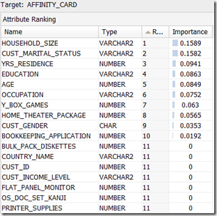
After everything has run, we get the little green box with the tick mark on the Filter Column node. To view the results we right clicking on the Filter Columns node and select View Data from the menu. We get the list of attributes listed in order of importance and their Importance measure.

image

We see that there are a number of attributes that have a zero value. It algorithm has worked out that these attributes would not be used in the model build step. If we look back to the previous blog post, some of the attributes we identified in it have also been listed here with a zero value.

Tuesday, January 3, 2012

ODM 11gR2–Using different data sources for Build and Testing a Model

There are 2 ways to connect a data source to the Model build node in Oracle Data Miner.

The typical method is to use a single data source that contains the data for the build and testing stages of the Model Build node. Using this method you can specify what percentage of the data, in the data source, to use for the Build step and the remaining records will be used for testing the model. The default is a 50:50 split but you can change this to what ever percentage that you think is appropriate (e.g. 60:40). The records will be split randomly into the Built and Test data sets.

image

The second way to specify the data sources is to use a separate data source for the Build and a separate data source for the Testing of the model.

To do this you add a new data source (containing the test data set) to the Model Build node. ODM will assign a label (Test) to the connector for the second data source.

image

If the label was assigned incorrectly you can swap what data sources. To do this right click on the Model Build node and select Swap Data Sources from the menu.

image

image

Tuesday, December 20, 2011

Updating your ODM (11g R2) model in production

In my previous blog posts on creating an ODM model, I gave the details of how you can do this using the ODM PL/SQL API.

But at some point you will have a fairly stable environment. What this means is that you will know what type of algorithm and its corresponding settings work best for for your data.

At this point you should be able to re-create your ODM model in the production database. The frequency of doing this update is dependent on number of new cases that you have. So you need to update your ODM model could be daily, weekly, monthly, etc.

image

To update your model you will need to:

- Creating a settings table for your model
- Create a new ODM model
- Rename your new ODM model to the production name

The following examples are based on the example data, model names, etc that I’ve used in my previous post.

Creating a Settings Table

The first step is to create a setting table for your algorithm. This will contain all the parameter settings needed to create the new model. You will have worked out these setting from your previous attempts at creating your models and you will know what parameters and their values work best.

-- Create the settings table
CREATE TABLE decision_tree_model_settings (
    setting_name VARCHAR2(30),
    setting_value VARCHAR2(30));

-- Populate the settings table
-- Specify DT. By default, Naive Bayes is used for classification.
-- Specify ADP. By default, ADP is not used.
BEGIN
    INSERT INTO decision_tree_model_settings (setting_name, setting_value)
    VALUES (dbms_data_mining.algo_name,       
           dbms_data_mining.algo_decision_tree);
   
    INSERT INTO decision_tree_model_settings (setting_name, setting_value)
    VALUES (dbms_data_mining.prep_auto,dbms_data_mining.prep_auto_on);
  
    COMMIT;
END;

Create a new ODM Model

We will need to use the DBMS_DATA_MINING.CREATE_MODEL procedure. In our example we will want to create a Decision Tree based on our sample data, which contains the previously generated cases and the new cases since the last model rebuild.

BEGIN
    DBMS_DATA_MINING.CREATE_MODEL(
        model_name          => ‘Decision_Tree_Method2',
        mining_function     => dbms_data_mining.classification,
        data_table_name     => 'mining_data_build_v',
        case_id_column_name => 'cust_id',
        target_column_name  => 'affinity_card',
        settings_table_name => ‘decision_tree_model_settings');
END;

Rename your ODM model to production name

The model we have create created above is not the name that is used in our production software. So we will need to rename it to our production name.

But we need to be careful about when we do this. If you drop a model or rename a model when it is being used then you can end up with indeterminate results.

What I suggest you do, is to pick a time of the day when your production software is not doing any data mining. You should drop the existing mode (or rename it) and the to rename the new model to the production model name.

DBMS_DATA_MINING.DROP_MODEL('CLAS_DECISION_TREE‘);

and then

DBMS_DATA_MINING.RENAME_MODEL('Decision_Tree_Method2', 'CLAS_DECISION_TREE');

Monday, December 19, 2011

Oracle Analytics Update & Plan for 2012

On Friday 16th December, Charlie Berger (Sr. Director, Product Management, Data Mining & Advanced Analytics) posted the following on the Oracle Data Mining forum on OTN.

“… soon you'll be able to use the new Oracle R Enterprise (ORE) functionality. ORE is currently in beta and is targeted to go General Availability in the near future. ORE brings additional functionality to the ODM Option, which will then be renamed to the Oracle Advanced Analytics Option to reflect the significant adv. analytical functionality enhancements. ORE will allow R users to write R scripts and run them inside the database and eliminate and/or minimize data movement in/out of the DB. ORE will provide R to SQL transparency for SQL push-down to in-DB SQL and and expanding library of Oracle in-DB statistical functions. Packages that cannot be pushed down will be run in embedded R mode while the DB manages all data flows to the multiple R engines running inside the DB.


In January, we'll open up a new OTN discussion forum specifically for Oracle R Enterprise focused technical discussions. Stay tuned.

I’m looking forward to getting my hands on the new Oracle R Enterprise, in 2012. In particular I’m keen to see what additional functionality will be added to the Oracle Data Mining option in the DB.

So watch out for the rebranding to Oracle Advanced Analytics

Charlie – Any chance of an advanced copy of ORE and related DB bits and bobs.

Monday, December 12, 2011

My UKOUG Presentation on ODM PL/SQL API

On Wednesday 7th Dec I gave my presentation at the UKOUG conference in Birmingham. The main topic of the presentation was on using the Oracle Data Miner PL/SQL API to implement a model in a production environment.

There was a good turn out considering it was the afternoon of the last day of the conference.

I asked the attendees about their experience of using the current and previous versions of the Oracle Data Mining tool. Only one of the attendees had used the pre 11g R2 version of the tool.

From my discussions with the attendees, it looks like they would have preferred an introduction/overview type presentation of the new ODM tool. I had submitted a presentation on this, but sadly it was not accepted.  Not enough people had voted for it.

For for next year, I will submit an introduction/overview presentation again, but I need more people to vote for it. So watch out for the vote stage next June and vote of it.

Here are the links to the presentation and the demo scripts (which I didn’t get time to run)

My Presentation

Demo Script 1 – Exploring and Exporting model

Demo Script 2 – Import, Dropping and Renaming the model. Plus Queries that use the model

Wednesday, November 9, 2011

ODM–PL/SQL API for Exporting & Importing Models

In a previous blog post I talked about how you can take a copy of a workflow developed in Oracle Data Miner, and load it into a new schema.
When you data mining project gets to a mature stage and you need to productionalise the data mining process and model updates, you will need to use a different set of tools.

As you gather more and more data and cases, you will be updating/refreshing your models to reflect this new data. The new update data mining model needs to be moved from the development/test environment to the production environment. As with all things in IT we would like to automate this updating of the model in production.
There are a number of database features and packages that we can use to automate the update and it involves the setting up of some scripts on the development/test database and also on the production database.

These steps include:

  • Creation of a directory on the development/test database
  • Exporting of the updated Data Mining model
  • Copying of the exported Data Mining model to the production server
  • Removing the existing Data Mining model from production
  • Importing of the new Data Mining model.
  • Rename the imported mode to the standard name

The DBMS_DATA_MINING PL/SQL package has 2 functions that allow us to export a model and to import a model. These functions are an API to the Oracle Data Pump. The function to export a model is DBMS_DATA_MINING.EXPORT_MODEL and the function to import a model is DBMS_DATA_MINING.IMPORT_MODEL.The parameters to these function are what you would expect use if you were to use Data Pump directly, but have been tailored for the data mining models.

Lets start with listing the models that we have in our development/test schema:

SQL> connect dmuser2/dmuser2
Connected.
SQL> SELECT model_name FROM user_mining_models;

MODEL_NAME
------------------------------
CLAS_DT_1_6
CLAS_SVM_1_6
CLAS_NB_1_6
CLAS_GLM_1_6

Create/define the directory on the server where the models will be exported to.

CREATE OR REPLACE DIRECTORY DataMiningDir_Exports AS 'c:\app\Data_Mining_Exports';

The schema you are using will need to have the CREATE ANY DIRECTORY privilege.

Now we can export our mode. In this example we are going to export the Decision Tree model (CLAS_DT_1_6)

DBMS_DATA_MINING.EXPORT_MODEL function
The function has the following structure

DBMS_DATA_MINING.EXPORT_MODEL (
     filename IN VARCHAR2,
     directory IN VARCHAR2,
     model_filter IN VARCHAR2 DEFAULT NULL,
     filesize IN VARCHAR2 DEFAULT NULL,
     operation IN VARCHAR2 DEFAULT NULL,
     remote_link IN VARCHAR2 DEFAULT NULL,
     jobname IN VARCHAR2 DEFAULT NULL);

If we wanted to export all the models into a file called Exported_DM_Models, we would run:

DBMS_DATA_MINING.EXPORT_MODEL('Exported_DM_Models', 'DataMiningDir');

If we just wanted to export our Decision Tree model to file Exported_CLASS_DT_Model, we would run:

DBMS_DATA_MINING.EXPORT_MODEL('Exported_CLASS_DT_Model', 'DataMiningDir', 'name in (''CLAS_DT_1_6'')');

DBMS_DATA_MINING.DROP_MODEL function
Before you can load the new update data mining model into your production database we need to drop the existing model. Before we do this we need to ensure that this is done when the model is not in use, so it would be advisable to schedule the dropping of the model during a quiet time, like before or after the nightly backups/processes.

DBMS_DATA_MINING.DROP_MODEL('CLAS_DECISION_TREE', TRUE)

DBMS_DATA_MINING.IMPORT_MODEL function
Warning : When importing the data mining model, you need to import into a tablespace that has the same name as the tablespace in the development/test database.  If the USERS tablespace is used in the development/test database, then the model will be imported into the USERS tablespace in the production database.

Hint : Create a DATAMINING tablespace in your development/test and production databases. This tablespace can be used solely for data mining purposes.

To import the decision tree model we exported previously, we would run

DBMS_DATA_MINING.IMPORT_MODEL('Exported_CLASS_DT_Model', 'DataMiningDir', 'name=’CLAS_DT_1_6''', 'IMPORT', null, null, 'dmuser2:dmuser3');

We now have the new updated data mining model loaded into the production database.

DBMS_DATA_MINING.RENAME_MODEL function
The final step before we can start using the new updated model in our production database is to rename the imported model to the standard name that is being used in the production database.

DBMS_DATA_MINING.RENAME_MODEL('CLAS_DT_1_6', 'CLAS_DECISION_TREE');

Scheduling of these steps
We can wrap most of this up into stored procedures and have schedule it to run on a semi-regular bases, using the DBMS_JOB function. The following example schedules a procedure that controls the importing, dropping and renaming of the models.

DBMS_JOB.SUBMIT(jobnum.nextval, 'import_new_data_mining_model', trunc(sysdate), add_month(trunc(sysdate)+1);

This schedules the the running of the procedure to import the new data mining models, to run immediately and then to run every month.

Thursday, November 3, 2011

ODM 11.2 Data Dictionary Views.

The Oracle 11.2 database contains the following Oracle Data Mining views. These allow you to query the database for the metadata relating to what Data Mining Models you have, what the configurations area and what data is involved.

ALL_MINING_MODELS

Describes the high level information about the data mining models in the database.  Related views include DBA_MINING_MODELS and USER_MINING_MODELS.

Attribute Data Type Description
OWNER Varchar2(30) NN Owner of the mining model
MODEL_NAME Varchar2(30) NN Name of the mining model
MINING_FUNCTION Varchar2(30) What data mining function to use
CLASSIFICATION
REGRESSION
CLUSTERING
FEATURE_EXTRACTION
ASSOCIATION_RULES
ATTRIBUTE_IMPORTANCE
ALGORITHM Varchar2(30) Algorithm used by the model
NAIVE_BAYES
ADAPTIVE_BAYES_NETWORK
DECISION_TREE
SUPPORT_VECTOR_MACHINES
KMEANS
O_CLUSTER
NONNEGATIVE_MATRIX_FACTOR
GENERALIZED_LINEAR_MODEL
APRIORI_ASSOCIATION_RULES
MINIMUM_DESCRIPTION_LENGTH
CREATION_DATE Date NN Date model was created
BUILD_DURATION Number Time in seconds for the model build process
MODEL_SIZE Number Size of model in MBytes
COMMENTS Varchar2(4000)  
Lets query the my DMUSER2 data mining schema. This was created during a previous post where we exported some ODM models from schema and loaded them into DMUSER2 schema

SELECT model_name, 
       mining_function,
       algorithm,
       build_duration,
       model_size
FROM ALL_MINING_MODELS;

MODEL_NAME     MINING_FUNCTION  ALGORITHM                      BUILD_DURATION MODEL_SIZE
-------------  ---------------- -------------------------- -------------- ----------
CLAS_SVM_1_6   CLASSIFICATION    SUPPORT_VECTOR_MACHINES                     3      .1515
CLAS_DT_1_6    CLASSIFICATION    DECISION_TREE                               2      .0842
CLAS_GLM_1_6   CLASSIFICATION    GENERALIZED_LINEAR_MODEL                    3      .0877
CLAS_NB_1_6    CLASSIFICATION    NAIVE_BAYES                                 2      .0459

ALL_MINING_MODEL_ATTRIBUTES

Describes the attributes of the data mining models.  Related views are DBA_MINING_MODEL_ATTRIBUTES and USER_MINING_MODEL_ATTRIBUTES.

Attribute Data Type Description
OWNER Varchar2(30) NN Owner of the mining model
MODEL_NAME Varchar2(30) NN Name of the mining mode
ATTRIBUTE_NAME Varchar2(30) NN Name of the attribute
ATTRIBUTE_TYPE Varchar2(11) Logical type of attribute
NUMERICAL – numeric data
CATEGORICAL – character data
DATA_TYPE Varchar2(12) Data type of attribute
DATA_LENGTH Number Length of data type
DATA_PRECISION Number Precision of a fixed point number
DATA_SCALE Number Scale of the fixed point number
USAGE_TYPE Varchar2(8) Indicated if the attribute was used to create the model (ACTIVE) or not (INACTIVE)
TARGET Varchar2(3) Indicates if the attribute is the target

If we take one of our data mining models that was listed about and select what attributes are used by that model;

SELECT attribute_name,
       attribute_type,
       usage_type,
       target
from all_mining_model_attributes
where model_name = 'CLAS_DT_1_6';

ATTRIBUTE_NAME                 ATTRIBUTE_T USAGE_TY TAR
------------------------------ ----------- -------- ---
AGE                            NUMERICAL   ACTIVE   NO
CUST_MARITAL_STATUS            CATEGORICAL ACTIVE   NO
EDUCATION                      CATEGORICAL ACTIVE   NO
HOUSEHOLD_SIZE                 CATEGORICAL ACTIVE   NO
OCCUPATION                     CATEGORICAL ACTIVE   NO
YRS_RESIDENCE                  NUMERICAL   ACTIVE   NO
Y_BOX_GAMES                    NUMERICAL   ACTIVE   NO
AFFINITY_CARD                  CATEGORICAL ACTIVE   YES

The first thing to note here is that all the attributes are listed as ACTIVE. This is the default and will be the case for all attributes for all the algorithms, so we can ignore this attribute in our queries, but it is good to check just in case.

The second thing to note is for the last row we have the AFFINITY_CARD has a target attribute value of YES. This is the target attributes used by the classification algorithm.

ALL_MINING_MODEL_SETTINGS

Describes the setting of the data mining models. The settings associated with a model are algorithm dependent. The Setting values can be provided as input to the model build process. Alternatively, separate settings table can used.  If no setting values are defined of provided, then the algorithm will use its default settings.

Attribute Data Type Description
OWNER Varchar2(30) NN Owner of the mining model
MODEL_NAME Varchar2(30) NN Name of the mining model
SETTING_NAME Varchar2(30) NN Name of the Setting
SETTING_VALUE Varchar2(4000) Value of the Setting
SETTING_TYPE Varchar2(7) Indicates whether the default value (DEFAULT) or a user specified value (INPUT) is used by the model

Lets take our previous example of the 'CLAS_DT_1_6' model and query the database to see what the setting are.

column setting_value format a30
select setting_name, 
       setting_value,
       setting_type
from all_mining_model_settings
where model_name = 'CLAS_DT_1_6';

SETTING_NAME            SETTING_VALUE                SETTING
----------------------- ---------------------------- -------
ALGO_NAME               ALGO_DECISION_TREE           INPUT
PREP_AUTO               ON                           INPUT
TREE_TERM_MINPCT_NODE   .05                          INPUT
TREE_TERM_MINREC_SPLIT  20                           INPUT
TREE_IMPURITY_METRIC    TREE_IMPURITY_GINI           INPUT
CLAS_COST_TABLE_NAME    ODMR$15_42_50_762000JERWZYK  INPUT
TREE_TERM_MINPCT_SPLIT  .1                           INPUT
TREE_TERM_MAX_DEPTH     7                            INPUT
TREE_TERM_MINREC_NODE   10                           INPUT

Monday, October 31, 2011

ODM 11.2–Data Mining PL/SQL Packages

The Oracle 11.2 database contains 3 PL/SQL packages that allow you to perform all (well almost all) of your data mining functions.

So instead of using the Oracle Data Miner tool you can write some PL/SQL code that will you to do the same things.

Before you can start using these PL/SQL packages you need to ensure that the schema that you are going to use has been setup with the following:

  • Create a schema or use and existing one
  • Grant the schema all the data mining privileges: see my earlier posting on how to setup an Oracle schema for data mining – Click here and YouTube video
  • Grant all necessary privileges to the data that you will be using for data mining

The first PL/SQL package that you will use is the DBMS_DATA_MINING_TRANSFORM. This PL/SQL package allows you to transform the data to make it suitable for data mining. There are a number of functions in this package that allows you to transform the data, but depending on the data you may need to write your own code to perform the transformations. When you apply your data model to the test or the apply data sets, ODM will automatically take the transformation functions defined using this package and apply them to the new data sets.

The second PL/SQL package is DBMS_DATA_MINING. This is the main data mining PL/SQL package. It contains functions to allow you to:

  • To create a Model
  • Describe the Model
  • Exploring and importing of Models
  • Computing costs and text metrics for classification Models
  • Applying the Model to new data
  • Administration of Models, like dropping, renaming, etc

The next (and last) PL/SQL package is DBMS_PREDICTIVE_ANALYTICS.The routines included in this package allows you to prepare data, build a model, score a model and return results of model scoring. The routines include EXPLAIN which ranks attributes in order of influence in explaining a target column. PREDICT which predicts the value of a target attribute based on values in the input. PROFILE which generates rules that describe the cases from the input data.

Over the coming weeks I will have separate blog posts on each of these PL/SQL packages. These will cover the functions that are part of each packages and will include some examples of using the package and functions.

Saturday, October 29, 2011

ODM PL/SQL API 11.2 New Features

The PL/SQL API interface for Oracle Data Miner has had a number of new features. These are listed below along with the new API features added with the 11.1 release.

  • Support for Native Transactional Data with Association Rules: you can build association rule models without first transforming the transactional data.
  • SVM class weights specified with CLAS_WEIGHTS_TABLE_NAME: including the GLM class weights
  • FORCE argument to DROP_MODEL: you can now force a drop model operation even if a serious system error has interrupted the model build process
  • GET_MODEL_DETAILS_SVM has a new REVERSE_COEF parameter: you can obtain the transformed attribute coefficients used internally by an SVM model by setting the new REVERSE_COEF parameter to 1

11.1g API New Features

  • Mining Model schema objects: previous releases, DM models were implemented as a collection of tables and metadata within the DMSYS schema. in 11.1 models are implemented as data dictionary objects in the SYS schema. A new set of DD views present DM models and their properties
  • Automatic and Embedded Data Preparation: previously data preparation was the responsibility of the user. Now it can be automated
  • Scoping of Nested Data: supports nested data types for both categorical and numerical data. Most algorithms require multi-record case data to the presented as columns of nested rows, each containing an attribute name/value pair. ODM processes each nested row as a separate attribute.
  • Standardised Handling of Sparse Data & Missing Values: standardised across all algorithms.
  • Generalised Linear Models: has a new algorithm and supports classification (logistic regression) and regression (linear regression)
  • New SQL Data Mining Function: PREDICTION_BOUNDS has been introduced for Generalised Linear Models. This returns the confidence bounds on predicted values (regression models) or predicted probabilities (classification)
  • Enhanced Support for Cost-Sensitive Decision Making: can be added or removed using DATA_MINING.ADD_COST_MATRIX and DBMS_DATA_MINING_REMOVE_COST_MATRIX.

Wednesday, October 19, 2011

ODM API Demos in PL/SQL (& Java)

If you have been using Oracle Data Miner to develop your data mining workflows and models, at some point you will want to move away from the tool and start using the ODM APIs.

Oracle Data Mining provides a PL/SQL API and a Java API for creating supervised and unsupervised data mining models. The two APIs are fully interoperable, so that a model can be created with one API and then modified or applied using the other API.

I will cover the Java APIs in a later post, so watch out for that.

To help you get started with using the APIs there are a number of demo PL/SQL programs available. These were available as part of the the pre-11.2g version of the tool. But they don’t seem to packaged up with the 11.2 (SQL Developer 3) application.

The following table gives a list of the PL/SQL demo programs that are available. Although these were part of the pre-11.2g tool, they still seem to work on your 11.2g database.

You can download a zip of these files from here.

The sample PL/SQL programs illustrate each of the algorithms supported by Oracle Data Mining. They include examples of data transformations appropriate for each algorithm.

image

I will be exploring the main APIs, how to set them up, the parameters, etc.,  over the next few weeks, so check back for these posts.