R vs Python vs SQL for Machine Learning (Infographic)

Next week I'll be giving several presentation on machine learning at Oracle Open World and Oracle Code One. In one of these presentation an evaluation of using R vs Python vs SQL will be given and discussed.

Check out the infographic containing the comparisons.

Click here to download the PDF version.

My book on Oracle R Enterprise translated into Chinese

A couple of days ago the post man knocked on my door with a package. I hadn't ordered anything, so it was a puzzling what it might be.

When I opened the package I found 3 copies of a book in Chinese.

It was one of my books !

One of my books was translated into Chinese !

What a surprise, as I wasn't aware this was happening.

At this time I'm not sure where you can purchase the book, but I'll update this blog post when I find out.

PRECIS R package

If you use R then you are very familiar with the SUMMARY function.

If you use R then you are very familiar with the name Hadley Wickham. He has produced some really cool packages for R.

He has produced a new R package and function that complements the commonly used SUMMARY R function.

The following outlines how you can install this new R package from GitHub (Hadley's GitHub is https://github.com/hadley/).

Install the R devtools package. This will allow you to download the package code from GitHub.

install.packages("devtools")

Install the package from Hadley's GitHub repository.

devtools::install_github("hadley/precis")

Load the library.

library(precis)

The following displays information produced by the SUMMARY and the PRECIS function.

> summary(mtcars)
      mpg             cyl             disp             hp             drat             wt       
 Min.   :10.40   Min.   :4.000   Min.   : 71.1   Min.   : 52.0   Min.   :2.760   Min.   :1.513  
 1st Qu.:15.43   1st Qu.:4.000   1st Qu.:120.8   1st Qu.: 96.5   1st Qu.:3.080   1st Qu.:2.581  
 Median :19.20   Median :6.000   Median :196.3   Median :123.0   Median :3.695   Median :3.325  
 Mean   :20.09   Mean   :6.188   Mean   :230.7   Mean   :146.7   Mean   :3.597   Mean   :3.217  
 3rd Qu.:22.80   3rd Qu.:8.000   3rd Qu.:326.0   3rd Qu.:180.0   3rd Qu.:3.920   3rd Qu.:3.610  
 Max.   :33.90   Max.   :8.000   Max.   :472.0   Max.   :335.0   Max.   :4.930   Max.   :5.424  
      qsec             vs               am              gear            carb      
 Min.   :14.50   Min.   :0.0000   Min.   :0.0000   Min.   :3.000   Min.   :1.000  
 1st Qu.:16.89   1st Qu.:0.0000   1st Qu.:0.0000   1st Qu.:3.000   1st Qu.:2.000  
 Median :17.71   Median :0.0000   Median :0.0000   Median :4.000   Median :2.000  
 Mean   :17.85   Mean   :0.4375   Mean   :0.4062   Mean   :3.688   Mean   :2.812  
 3rd Qu.:18.90   3rd Qu.:1.0000   3rd Qu.:1.0000   3rd Qu.:4.000   3rd Qu.:4.000  
 Max.   :22.90   Max.   :1.0000   Max.   :1.0000   Max.   :5.000   Max.   :8.000  
> precis(mtcars)
# data.frame [32 x 11]
    name  type                            precis
                                 
1    mpg   dbl  10.4 [ 15.4 ( 19.2)  22.8]  33.9
2    cyl   dbl               4 (11) 6 (7) 8 (14)
3   disp   dbl  71.1 [121.0 (196.0) 334.0] 472.0
4     hp   dbl    52 [   96 (  123)   180]   335
5   drat   dbl  2.76 [ 3.08 ( 3.70)  3.92]  4.93
6     wt   dbl  1.51 [ 2.54 ( 3.32)  3.65]  5.42
7   qsec   dbl  14.5 [ 16.9 ( 17.7)  18.9]  22.9
8     vs   dbl                     0 (18) 1 (14)
9     am   dbl                     0 (19) 1 (13)
10  gear   dbl               3 (15) 4 (12) 5 (5)
11  carb   dbl     1 [    2 (    2)     4]     8
> precis(mtcars, histogram=TRUE)
# data.frame [32 x 11]
    name  type                            precis
                                 
1    mpg   dbl           10.4 ▂▁▇▃▅▅▂▂▁▁▂▂  33.9
2    cyl   dbl      4 ▅▁▁▁▁▁▁▁▁▃▁▁▁▁▁▁▁▁▁▇     8
3   disp   dbl  71.1 ▅▁▁▃▇▂▁▁▁▁▃▁▃▁▅▁▁▁▁▁▁ 472.0
4     hp   dbl          52 ▁▅▅▇▂▂▇▁▂▁▂▁▁▁▁   335
5   drat   dbl           2.76 ▂▂▇▂▁▅▇▃▂▁▁▁  4.93
6     wt   dbl  1.51 ▁▁▂▂▁▁▂▁▂▁▇▂▂▁▁▁▁▁▁▂▁  5.42
7   qsec   dbl      14.5 ▂▂▁▁▃▇▅▁▇▂▂▂▁▁▁▁▁  22.9
8     vs   dbl      0 ▇▁▁▁▁▁▁▁▁▁▁▁▁▁▁▁▁▁▁▅     1
9     am   dbl      0 ▇▁▁▁▁▁▁▁▁▁▁▁▁▁▁▁▁▁▁▅     1
10  gear   dbl      3 ▇▁▁▁▁▁▁▁▁▅▁▁▁▁▁▁▁▁▁▂     5
11  carb   dbl            1 ▅▇▁▂▁▇▁▁▁▁▁▁▁▁     8
 

Managing memory allocation for Oracle R Enterprise Embedded Execution

When working with Oracle R Enterprise and particularly when you are using the ORE functions that can spawn multiple R processes, on the DB Server, you need to be very aware of the amount of memory that will be consumed for each call of the ORE function.

ORE has two sets of parallel functions for running your user defined R scripts stored in the database, as part of the Embedded R Execution feature of ORE. The R functions are called ore.groupApply, ore.rowApply and ore.indexApply. When using SQL there are "rqGroupApply" and rqRowApply. (There is no SQL function equivalent of the R function ore.indexApply)

For each parallel R process that is spawned on the DB server a certain amount of memory (RAM) will be allocated to this R process. The default size of memory to be allocated can be found by using the following query.

select name, value from sys.rq_config;

NAME                                VALUE
----------------------------------- -----------------------------------
VERSION                             1.5
MIN_VSIZE                           32M
MAX_VSIZE                           4G
MIN_NSIZE                           2M
MAX_NSIZE                           20M

The memory allocation is broken out into the amount of memory allocated for Cells and NCells for each R process.

If your parallel ORE function create a large number of parallel R processes then you can see that the amount of overall memory consumed can be significant. I've seen a few customers who very quickly run out of memory on their DB servers. Now that is something you do not want to happen.

How can you prevent this from happening ?

There are a few things you need to keep in mind when using the parallel enabled ORE functions. The first one is, how many R processes will be spawned. For most cases this can be estimated or calculated to a high degree of accuracy. Secondly, how much memory will be used to process each of the R processes. Thirdly, how memory do you have available on the DB server. Fourthly, how many other people will be running parallel R processes at the same time?

Examining and answering each of these may look to be a relatively trivial task, but the complexity behind these can increase dramatically depending on the answer to the fourth point/question above.

To calculate the amount of memory used during the ORE user defined R script, you can use the R garbage function to calculate the memory usage at the start and at the end of the R script, and then return the calculated amount. Yes you need to add this extra code to your R script and then remove it when you have calculated the memory usage.

gc.start <- gc(reset=TRUE)
...
gc.end <- gc()
gc.used <- gc.end[,7] - gc.start[,7] # amount consumed by the processing

Using this information and the answers to the points/questions I listed above you can now look at calculating how much memory you need to allocated to the R processes. You can set this to be static for all R processes or you can use some code to allocate the amount of memory that is needed for each R process. But this starts to become messy. The following gives some examples (using R) of changing the R memory allocations in the Oracle Database. Similar commands can be issued using SQL.

> sys.rqconfigset('MIN_VSIZE', '10M') -- min heap 10MB, default 32MB
> sys.rqconfigset('MAX_VSIZE', '100M') -- max heap 100MB, default 4GB
> sys.rqconfigset('MIN_NSIZE', '500K') -- min number cons cells 500x1024, default 1M
> sys.rqconfigset('MAX_NSIZE', '2M') -- max number cons cells 2M, default 20M

Some guidelines - as with all guidelines you have to consider all the other requirements for the Database, and in reality you will have to try to find a balance between what is listed here and what is actually possible.

• Set parallel_degree_policy to MANUAL.
• Set parallel_min_servers to the number of parallel slave processes to be started when the database instances start, this avoids start up time for the R processes. This is not a problem for long running processes. But can save time with processes running for 10s seconds
• To avoid overloading the CPUs if the parallel_max_servers limit is reached, set the hidden parameter _parallel_statement_queuing to TRUE. Avoids overloading and lets processes wait.
• Set application tables and their indexes to DOP 1 to reinforce the ability of ORE to determine when to use parallelism.

Understanding the memory requirements for your ORE processes can be tricky business and can take some time to work out the right balance between what is needed by the spawned parallel R processes and everything else that is going on in the Database. There will be a lot of trial and error in working this out and it is always good to reach out for some help. If you have a similar scenario and need some help or guidance let me know.

OUG Ireland 2017 Presentation

Here are the slides from my presentation at OUG Ireland 2017. All about running R using SQL.

Embedded R Execution using SQL from Brendan Tierney

Formatting results from ORE script in a SELECT statement

This blog post looks at how to format the output or the returned returns from an Oracle R Enterprise (ORE), user defined R function, that is run using a SELECT statement in SQL.

Sometimes this can be a bit of a challenge to work out, but it can be relatively easy once you have figured out how to do it. The following examples works through some scenarios of different results sets from a user defined R function that is stored in the Oracle Database.

To run that user defined R function using a SELECT statement I can use one of the following ORE SQL functions.

• rqEval
• rqTableEval
• "rqGroupEval"
• rqRowEval

For simplicity we will just use the first of these ORE SQL functions to illustrate the problem and how to go about solving it. The rqEval ORE SQL function is a generate purpose function to call a user defined R script stored in the database. The function does not require any input data set and but it will return some data. You could use this to generate some dummy/test data or to find some information in the database. Here is noddy example that returns my name.

BEGIN
   --sys.rqScriptDrop('GET_NAME');
   sys.rqScriptCreate('GET_NAME',
      'function() {
         res<-data.frame("Brendan")
         res
         } ');
END;

To call this user defined R function I can use the following SQL.

select *
from table(rqEval(null,
                  'select cast(''a'' as varchar2(50))  from dual',
                  'GET_NAME') );  

For text strings returned you need to cast the returned value giving a size.

If we have a numeric value being returned we can don't have to use the cast and instead use '1' as shown in the following example. This second example extends our user defined R function to return my name and a number.

BEGIN
   sys.rqScriptDrop('GET_NAME');
   sys.rqScriptCreate('GET_NAME',
      'function() {
         res<-data.frame(NAME="Brendan", YEAR=2017)
         res
         } ');
END;

To call the updated GET_NAME function we now have to process two returned columns. The first is the character string and the second is a numeric.

select *
from table(rqEval(null,
                  'select cast(''a'' as varchar2(50)) as "NAME", 1 AS YEAR  from dual',
                  'GET_NAME') );                  

These example illustrate how you can process character strings and numerics being returned by the user defined R script.

The key to setting up the format of the returned values is knowing the structure of the data frame being returned by the user defined R script. Once you know that the rest is (in theory) easy.

Creating and Reading SPSS and SAS data sets in R

NOTE: Several people have contacted me to say that using this R package does not work. The data set 
generated is not readable by SAS. If you encounter this problem then get in touch with the creators 
of Haven for help and support. I'm using R version 3.2.0.
All I an say is, it worked for me!

Have you ever been faced with having to generate a data set in the format that is needed by another analytics tool? or having to generate a data set in a particular format but you don't have the software that generates that format? For example, if you are submitting data to the FDA and other bodies, you may need to submit the data in a SAS formatted file. There are a few ways you can go about this.

One option is that you can use the Haven R package to generate your dataset in SAS and SPSS formats. But you can also read in SAS and SPSS formatted files. I have to deal with these formatted data files all the time, and it can be a challenge, but I've recently come across the Haven R package that has just made my life just a little bit/lots easier. Now I can easily generate SAS and SPSS formatted data sets for my data in my Oracle Database, using R and ORE. ORE we can now use the embedded feature to build the generation of these data sets into some of our end-user applications.

Let us have a look at Haven and what it can do.

Firstly there is very little if any documentation online for it. That is ok so we will have to rely on the documentation that comes with the R packages. Again there isn't much to help and that is because the R package mainly consists of functions to Read in these data sets, functions to Write these data sets and some additional functions for preparing data.

For reading in data sets we have the following functions:

# SAS
read_sas("mtcars.sas7bdat")
# Stata
read_dta("mtcars.dta")
# SPSS
read_sav("mtcars.sav")

For writing data sets we have the following functions:

# SAS
write_sas(mtcars, "mtcars.sas7bdat")
# Stata
write_dta(mtcars, "mtcars.dta")
# SPSS
write_sav(mtcars, "mtcars.sav")

Let us now work through an example of creating a SAS data set. We can use some of the sample data sets that come with the Oracle Database in the SH schema. I'm going to use the data in the CUSTOMER table to create a SAS data set. In the following code I'm using ORE to connect to the database but you can use your preferred method.

> library(ORE)
> # Create your connection to the schema in the DB
> ore.connect(user="sh", password="sh", host="localhost", service_name="PDB12C", 
            port=1521, all=TRUE) 

> dim(CUSTOMERS)
[1] 55500    23
> names(CUSTOMERS)
 [1] "CUST_ID"                "CUST_FIRST_NAME"        "CUST_LAST_NAME"        
 [4] "CUST_GENDER"            "CUST_YEAR_OF_BIRTH"     "CUST_MARITAL_STATUS"   
 [7] "CUST_STREET_ADDRESS"    "CUST_POSTAL_CODE"       "CUST_CITY"             
[10] "CUST_CITY_ID"           "CUST_STATE_PROVINCE"    "CUST_STATE_PROVINCE_ID"
[13] "COUNTRY_ID"             "CUST_MAIN_PHONE_NUMBER" "CUST_INCOME_LEVEL"     
[16] "CUST_CREDIT_LIMIT"      "CUST_EMAIL"             "CUST_TOTAL"            
[19] "CUST_TOTAL_ID"          "CUST_SRC_ID"            "CUST_EFF_FROM"         
[22] "CUST_EFF_TO"            "CUST_VALID"      

Next we can prepare the data, take a subset of the data, reformat the data, etc. For me I just want to use the data as it is. All I need to do now is to pull the data from the database to my local R environment.

dat <- ore.pull(CUSTOMERS)

Then I need to load the Haven library and then create the SAS formatted file.

library(haven)
write_sas(dat, "c:/app/my_customers.sas7bdat")

That's it. Nice and simple.

But has it worked? Has it created the file correctly? Will it load into my SAS tool?

There is only one way to test this and that is to only it in SAS. I have an account on SAS OnDemand with access to several SAS products. I'm going to use SAS Studio.

Well it works! The following image shows SAS Studio after I had loaded the data set with the variables and data shown.

WARNING: When you load the data set into SAS you may get a warning message saying that it isn't a SAS data set. What this means is that it is not a data set generated by SAS. But as you can see in the image above all the data got loaded OK and you can work away with it as normal in your SAS tools.

The next step is to test the loading of a SAS data set into R. I'm going to use one of the standard SAS data sets called PVA97NK.SAS7BDAT. If you have worked with SAS products then you will have come across this data set.

When you use Haven to load in your SAS data set, it will create the data in tribble format. This is a slight varient of a data.frame. So if you want the typical format of a data.frmae then you will need to convert the loaded data, as shown in the following code.

> data_read <- read_sas("c:/app/pva97nk.sas7bdat")
> dim(data_read)
[1] 9686   28
> d<-data.frame(data_read)
> class(data_read)
[1] "tbl_df"     "tbl"        "data.frame"
> class(d)
[1] "data.frame"
> head(d)
  TARGET_B       ID TARGET_D GiftCnt36 GiftCntAll GiftCntCard36 GiftCntCardAll
1        0 00014974       NA         2          4             1              3
2        0 00006294       NA         1          8             0              3
3        1 00046110        4         6         41             3             20
...

I think this package to going to make my life a little bit easier, and if you work with SPSS and SAS data sets then hopefully some of your tasks have become a little bit easier too.

Machine Learning notebooks (and Oracle)

Over the past 12 months there has been an increase in the number of Machine Learning notebooks becoming available.
What is a Machine Learning notebook?
As the name implies it can be used to perform machine learning using one or more languages and allows you to organise your code, scripts and other details in one application.
The ML notebooks provide an interactive environment (sometimes browser based) that allows you to write, run, view results, share/collaborate code and results, visualise data, etc.
Some of these ML notebooks come with one language and others come with two or more languages, and have the ability to add other ML related languages. The most common languages are Spark, Phython and R.
Based on these languages ML notebooks are typically used in the big data world and on Hadoop.

Examples of Machine Learning notebooks include: (Starting with the more common ones)

• Apache Zeppelin
• Jupyter Notebook (formally known as IPython Notebook)
• Azure ML R Notebook
• Beaker Notebook
• SageMath

At Oracle Open World (2016), Oracle announced that they are currently working creating their own ML notebook and it is based on Apache Zeppelin. They seemed to indicate that a beta version might be available in 2017. Here are some photos from that presentation, but with all things that Oracle talk about you have to remember and take into account their Safe Habor.

I'm looking forward to getting my hands on this new product when it is available.

Change the size of ORE PNG graphics using in-database R functions

In a previous blog post I showed you how create and display a ggplot2 R graphic using SQL. Make sure to check it out before reading the rest of this blog post.
In my previous blog post, I showed and mentioned that the PNG graphic returned by the embedded R execution SQL statement was not the same as what was produced if you created the graphic in an R session.
Here is the same ggplot2 graphic. The first one is what is produced in an R session and the section is what is produced by SQL query and the embedded R execution in Oracle.

As you can see the second image (produced using the embedded R execution) gives a very square image.
The reason for this is that Oracle R Enterprise (ORE) creates the graphic image in PNG format. The default setting from this is 480 x 480. You will find this information when you go digging in the R documentation and not in the Oracle documentation.
So, how can I get my ORE produced graphic to appear like what is produced in R?
What you need to do is to change the height and width of the PNG image produced by ORE. You can do this by passing parameters in the SQL statement used to call the user defined R function, that in turn produces the ggplot2 image.
In my previous post, I gave the SQL statement to call and produce the graphic (shown above). One of the parameters to the rqTableEval function was set to null. This was because we didn't have any parameters to pass, apart from the data set.
We can replace this null with any parameters we want to pass to the user defined R function (demo_ggpplot). To pass the parameters we need to define them using a SELECT statement.

cursor(select 500 as "ore.png.height", 850 as "ore.png.width" from dual),

The full SELECT statement now becomes

select *
from table(rqTableEval( cursor(select * from claims),
                        cursor(select 500 as "ore.png.height", 850 as "ore.png.width" from dual),
                        'PNG',
                        'demo_ggpplot'));

When you view the graphic in SQL Developer, you will get something that looks a bit more like what you would expect or want to see.

For each graphic image you want to produce using ORE you will need to figure out that are the best PNG height and width settings to use. Plus it also depends on what tool or application you are going to use to display the images (eg. APEX etc)

Oracle Text, Oracle R Enterprise and Oracle Data Mining - Part 2

This is the second blog post of a series on using Oracle Text, Oracle R Enterprise and Oracle Data Mining. Check out the first blog post of the series, as the data used in this blog post was extracted, processed and stored in a databases table.

In this blog post I will show you how you use Oracle R Enterprise and the embedded R execution features of ORE to use the text from the webpages and to create a word cloud. This is a useful tool to be able to see visually what words can stand out most on your webpage and if the correct message is being put across to your customers.

Prerequisites: You will need to load the following R packages into your R environment 'tm', 'word cloud' 'SnowballC'. These are required to process the following R code segments.

install.packages (c( "tm", "wordcloud", "SnowballC"))
library (tm)
library (wordcloud)
library (SnowballC)

Select data from table and prepare: We need to select the data from the table in our schema and to merge it into one variable.

local_data <- ore.pull(MY_DOCUMENTS)

tm_data <-""
for(i in 1:nrow(local_data)) {
  tm_data <- paste(tm_data, local_data[i,]$DOC_TEXT, sep=" ")
}
tm_data

Create function to perform Text Mining: In my previous blog post on creating a word cloud I gave the R code. In order to allow for this R code to be run on the database server (using the embedded R execution of ORE) we need to package this text mining R code up into a ORE user defined R script. This is stored in the database.

ore.scriptDrop("prepare_tm_data")
ore.scriptCreate("prepare_tm_data", function (tm_data) { 
  library(tm)
  library(SnowballC)
  library(wordcloud)
  
  txt_corpus <- Corpus (VectorSource (tm_data))
  
  # data clean up
  tm_map <- tm_map (txt_corpus, stripWhitespace) # remove white space
  tm_map <- tm_map (tm_map, removePunctuation) # remove punctuations
  tm_map <- tm_map (tm_map, removeNumbers) # to remove numbers
  tm_map <- tm_map (tm_map, removeWords, stopwords("english")) # to remove stop words
  tm_map <- tm_map (tm_map, removeWords, c("work", "use", "java", "new", "support"))
  
  # prepare matrix of words and frequency counts
  Matrix <- TermDocumentMatrix(tm_map) # terms in rows
  matrix_c <- as.matrix (Matrix)
  freq <- sort (rowSums (matrix_c)) # frequency data
  
  res <- data.frame(words=names(freq), freq)
  wordcloud (res$words, res$freq, max.words=100, min.freq=3, scale=c(7,.5), random.order=FALSE, colors=brewer.pal(8, "Dark2"))
} ) 

Before we can run this user define R script, we need to ensure that we have the 'tm', 'SnowballC' and 'wordcloud' R packages installed on the Oracle Database server. On the Oracle Database server you need to rune ORE.

> library(ORE)

Then run the following command to install these R packages

> install_packages(c('tm','wordcloud', 'SnowballC'))

Run the function on the DB Server: You are now ready to run the function. In an earlier step we had gathered the data. Now we can pass this data to the in-database R script.

> res <- ore.doEval(FUN.NAME="prepare_tm_data", tm_data=tm_data)

The ore.doEval function is a general purpose ORE function. In this case we pass it two parameters. The first parameter is the neame of the user defined R script stored in the database, and the second parameter is the data. The function returns and ORE object that contains the word cloud graphic.

Display the results: You can very easily display the results.

> res

This gives us the following graphic.

In my next blog post, of this series, I will show you how you can use the function created above and some other bits and pieces, using some other features of ORE and also in SQL.

Oracle Text, Oracle R Enterprise and Oracle Data Mining - Part 1

A project that I've been working on for a while now involves the use of Oracle Text, Oracle R Enterprise and Oracle Data Mining. Oracle Text comes with your Oracle Database licence. Oracle R Enterprise and Oracle Data Mining are part of the Oracle Advanced Analytics (extra cost) option.

What I will be doing over the course of 4 or maybe 5 blog posts is how these products can work together to help you gain a grater insight into your data, and part of your data being large text items like free format text, documents (in various forms e.g. html, xml, pdf, ms word), etc.

Unfortunately I cannot show you examples from the actual project I've been working on (and still am, from time to time). But what I can do is to show you how products and components can work together.

In this blog post I will just do some data setup. As with all project scenarios there can be many ways of performing the same tasks. Some might be better than others. But what I will be showing you is for demonstration purposes.

The scenario: The scenario for this blog post is that I want to extract text from some webpages and store them in a table in my schema. I then want to use Oracle Text to search the text from these webpages.

Schema setup: We need to create a table that will store the text from the webpages. We also want to create an Oracle Text index so that this text is searchable.

drop sequence my_doc_seq;
create sequence my_doc_seq;

drop table my_documents;

create table my_documents (
doc_pk number(10) primary key, 
doc_title varchar2(100), 
doc_extracted date, 
data_source varchar2(200), 
doc_text clob);

create index my_documents_ot_idx on my_documents(doc_text) 
indextype is CTXSYS.CONTEXT;

In the table we have a number of descriptive attributes and then a club for storing the website text. We will only be storing the website text and not the html document (More on that later). In order to make the website text searchable in the DOC_TEXT attribute we need to create an Oracle Text index of type CONTEXT.

There are a few challenges with using this type of index. For example when you insert a new record or update the DOC_TEXT attribute, the new values/text will not be reflected instantly, just like we are use to with traditional indexes. Instead you have to decide when you want to index to be updated. For example, if you would like the index to be updated after each commit then you can create the index using the following.

create index my_documents_ot_idx on my_documents(doc_text) 
indextype is CTXSYS.CONTEXT
parameters ('sync (on commit)');

Depending on the number of documents you have being committed to the DB, this might not be for you. You need to find the balance. Alternatively you could schedule the index to be updated by passing an interval to the 'sync' in the above command. Alternatively you might want to use DBMS_JOB to schedule the update.

To manually sync (or via DBMS_JOB) the index, assuming we used the first 'create index' statement, we would need to run the following.

EXEC CTX_DDL.SYNC_INDEX('my_documents_ot_idx');

This function just adds the new documents to the index. This can, over time, lead to some fragmentation of the index, and will require it to the re-organised on a semi-regular basis. Perhaps you can schedule this to happen every night, or once a week, or whatever makes sense to you.

BEGIN
  CTX_DDL.OPTIMIZE_INDEX('my_documents_ot_idx','FULL');
END;

(I could talk a lot more about setting up some basics of Oracle Text, the indexes, etc. But I'll leave that for another day or you can read some of the many blog posts that already exist on the topic.)

Extracting text from a webpage using R: Some time ago I wrote a blog post on using some of the text mining features and packages in R to produce a word cloud based on some of the Oracle Advanced Analytics webpages. I'm going to use the same webpages and some of the same code/functions/packages here. The first task you need to do is to get your hands on the 'htmlToText function. You can download the htmlToText function on github. This function requires the 'Curl' and 'XML' R packages. So you may need to install these. I also use the str_replace_all function ("stringer' R package) to remove some of the html that remains, to remove some special quotes and to replace and occurrences of '&' with 'and'. # Load the function and required R packages source("c:/app/htmltotext.R") library(stringr)

data1 <- str_replace_all(htmlToText("http://www.oracle.com/technetwork/database/options/advanced-analytics/overview/index.html"), "[\r\n\t\"\'\u201C\u201D]" , "")
data1 <- str_replace_all(data1, "&", "and")
data2 <- str_replace_all(str_replace_all(htmlToText("http://www.oracle.com/technetwork/database/options/advanced-analytics/odm/index.html"), "[\r\n\t\"\'\u201C\u201D]" , ""), "&", "and")
data2 <- str_replace_all(data2, "&", "and")
data3 <- str_replace_all(str_replace_all(htmlToText("http://www.oracle.com/technetwork/database/database-technologies/r/r-technologies/overview/index.html"), "[\r\n\t\"\'\u201C\u201D]" , ""), "&", "and")
data3 <- str_replace_all(data3, "&", "and")
data4 <- str_replace_all(str_replace_all(htmlToText("http://www.oracle.com/technetwork/database/database-technologies/r/r-enterprise/overview/index.html"), "[\r\n\t\"\'\u201C\u201D]" , ""), "&", "and")
data4 <- str_replace_all(data4, "&", "and")

We now have the text extracted and cleaned up. Create a data frame to contain all our data: Now that we have the text extracted, we can prepare the other data items we need to insert the data into our table ('my_documents'). The first stept is to construct a data frame to contain all the data.

data_source = c("http://www.oracle.com/technetwork/database/options/advanced-analytics/overview/index.html",
                 "http://www.oracle.com/technetwork/database/options/advanced-analytics/odm/index.html",
                 "http://www.oracle.com/technetwork/database/database-technologies/r/r-technologies/overview/index.html",
                 "http://www.oracle.com/technetwork/database/database-technologies/r/r-enterprise/overview/index.html")
doc_title = c("OAA_OVERVIEW", "OAA_ODM", "R_TECHNOLOGIES", "OAA_ORE")
doc_extracted = Sys.Date()
data_text <- c(data1, data2, data3, data4)

my_docs <- data.frame(doc_title, doc_extracted, data_source, data_text)

Insert the data into our database table: With the data in our data fram (my_docs) we can now use this data to insert into our database table. There are a number of ways of doing this in R. What I'm going to show you here is how to do it using Oracle R Enterprise (ORE). The thing with ORE is that there is no explicit functionality for inserting and updating records in a database table. What you need to do is to construct, in my case, the insert statement and then use ore.exec to execute this statement in the database.

library(ORE)
ore.connect(user="ora_text", password="ora_text", host="localhost", service_name="PDB12C", 
            port=1521, all=TRUE) 

for(i in 1:nrow(my_docs)) {
  insert_stmt <- "BEGIN insert_tab_document ('"
  insert_stmt <- paste(insert_stmt,  my_docs[i,]$doc_title, sep="")
  insert_stmt <- paste(insert_stmt, "', '",  my_docs[i,]$doc_extracted, "'", sep="")
  insert_stmt <- paste(insert_stmt, ", '",  my_docs[i,]$data_source, sep="")
  insert_stmt <- paste(insert_stmt, "', '",  my_docs[i,]$data_text, "');", " END;", sep="")
  ore.exec(insert_stmt)
}
ore.exec("commit")

You can now view the inserted webpage text using R or using SQL.

In my next blog post in this series, I will look at how you can use the ORE embedded features to read and process this data.

Creating ggplot2 graphics using SQL

Did you read the title of this blog post! Read it again.

Yes, Yes, I know what you are saying, "SQL cannot produce graphics or charts and particularly not ggplot2 graphics".

You are correct to a certain extent. SQL is rubbish a creating graphics (and I'm being polite).

But with Oracle R Enterprise you can now produce graphics on your data using the embedded R execution feature of Oracle R Enterprise using SQL. In this blog post I will show you how.

1. Pre-requisites

You need to have installed Oracle R Enterprise on your Oracle Database Server. Plus you need to install the ggplot2 R package.

In your R session you will need to setup a ORE connection to your Oracle schema.

2. Write and Test your R code to produce the graphic

It is always a good idea to write and test your R code before you go near using it in a user defined function.

For our (first) example we are going to create a bar chart using the ggplot2 R package. This is a basic example and the aim is to illustrate the steps you need to go through to call and produce this graphic using SQL.

The following code using the CLAIMS data set that is available with/for Oracle Advanced Analytics. The first step is to pull the data from the table in your Oracle schema to your R session. This is because ggplot2 cannot work with data referenced by an ore.frame object.

data.subset <- ore.pull(CLAIMS) 

Next we need to aggregate the data. Here we are counting the number of records for each Make of car.

aggdata2 <- aggregate(data.subset$POLICYNUMBER,
                      by = list(MAKE = data.subset$MAKE),
                      FUN = length)

Now load the ggplot2 R package and use it to build the bar chart.

ggplot(data=aggdata2, aes(x=MAKE, y=x, fill=MAKE)) + 
       geom_bar(color="black", stat="identity") +
       xlab("Make of Car") + 
       ylab("Num of Accidents") + 
       ggtitle("Accidents by Make of Car")

The following is the graphic that our call to ggplot2 produces in R.

At this point we have written and tested our R code and know that it works.

3. Create a user defined R function and store it in the Oracle Database

Our next step in the process is to create an in-database user defined R function. This is were we store R code in our Oracle Database and make this available as an R function. To create the user defined R function we can use some PL/SQL to define it, and then take our R code (see above) and in it.

BEGIN
   -- sys.rqScriptDrop('demo_ggpplot');
   sys.rqScriptCreate('demo_ggpplot', 
      'function(dat) {
         library(ggplot2)
         
         aggdata2 <- aggregate(dat$POLICYNUMBER,
                      by = list(MAKE = dat$MAKE),
                      FUN = length)

        g <-ggplot(data=aggdata2, aes(x=MAKE, y=x, fill=MAKE)) + geom_bar(color="black", stat="identity") +
                   xlab("Make of Car") + ylab("Num of Accidents") + ggtitle("Accidents by Make of Car")

        plot(g)
   }');
END;

We have to make a small addition to our R code. We need need to include a call to the plot function so that the image can be returned as a BLOB object. If you do not do this then the SQL query in step 4 will return no rows.

4. Write the SQL to call it

To call our defined R function we will need to use one of the ORE SQL API functions. In the following example we are using the rqTableEval function. The first parameter for this function passes in the data to be processed. In our case this is the data from the CLAIMS table. The second parameter is set to null. The third parameter is set to the output format and in our case we want this to be PNG. The fourth parameter is the name of the user defined R function.

select *
from table(rqTableEval( cursor(select * from claims),
                        null,
                        'PNG',
                        'demo_ggpplot'));                        

5. How to view the results

The SQL query in Step 4 above will return one row and this row will contain a column with a BLOB data type.

The easiest way to view the graphic that is produced is to use SQL Developer. It has an inbuilt feature that allows you to display BLOB objects. All you need to do is to double click on the BLOB cell (under the column labeled IMAGE). A window will open called 'View Value'. In this window click the 'View As Image' check box on the top right hand corner of the window. When you do the R ggplot2 graphic will be displayed.

Yes the image is not 100% the same as the image produced in our R session. I will have another blog post that deals with this at a later date.

But, now you have written a SQL query, that calls R code to produce an R graphic (using ggplot2) of our data.

6. Now you can enhance the graphics (without changing your SQL)

What if you get bored with the bar chart and you want to change it to a different type of graphic? All you need to do is to change the relevant code in the user defined R function.

For example, if we want to change the graphic to a polar plot. The following is the PL/SQL code that re-defines the user defined R script.

BEGIN
   sys.rqScriptDrop('demo_ggpplot');
   sys.rqScriptCreate('demo_ggpplot', 
      'function(dat) {
         library(ggplot2)
         
         aggdata2 <- aggregate(dat$POLICYNUMBER,
                      by = list(MAKE = dat$MAKE),
                      FUN = length)

         n <- nrow(aggdata2)
         degrees <- 360/n

        aggdata2$MAKE_ID <- 1:nrow(aggdata2)

        g<- ggplot(data=aggdata2, aes(x=MAKE, y=x, fill=MAKE)) + geom_bar(color="black", stat="identity") +
               xlab("Make of Car") + ylab("Num of Accidents") + ggtitle("Accidents by Make of Car") + coord_polar(theta="x") 
        plot(g)
   }');
END;

We can use the exact same SQL query we defined in Step 4 above to call the next graphic.

All done.

Now that was easy! Right?

I kind of is easy once you have been shown. There are a few challenges when working in-database user defined R functions and writing the SQL to call them. Most of the challenges are around the formatting of R code in the function and the syntax of the SQL statement to call it. With a bit of practice it does get easier.

7. Where/How can you use these graphics ?

Any application or program that can call and process a BLOB data type can display these images. For example, I've been able to include these graphics in applications developed in APEX.

googleVis R package for creating google charts in R

I've recently come across the 'googleVis' R package. This allows you to create a variety of different (typical and standard) charts in R but with the look and feel of the charts we can get from a number of different Google sites.

I won't bore you with some examples in the post but I'll point you to a good tutorial on the various charts.

Here is the link to the mini-tutorial.

Before you can use the package you will need to install it. The simplest way is to run the following in your R session.

> install.packages("googleVis")

Depending on your version of R you may need to upgrade.

Here is a selection of some of the charts you can create, and there are many, many more.

Some of you might be familiar with the presenting that Hans Rosling gives. Some of the same technology is behind these bubble charts from Google, as they bought the software years ago. Hans typically uses a data set that consists of GDP, Population and Life Expectancy for countries around the World. You too can use this same data set and is available from rdatamarket. The following R codes will extract this data set to you local R session and you can then use it as input to the various charts in the googleVis functions.

install.packages("rdatamarket")
library(rdatamarket)
dminit(NULL)

# Pull in life expectancy and population data
life_expectancy <- dmlist("15r2!hrp")
population <- dmlist("1cfl!r3d")

# Pull in the yearly GDP for each country
gdp <- dmlist("15c9!hd1")

# Load in the plyr package
library("plyr")

# Rename the Value for each dataset
names(gdp)[3] <- "GDP"

# Use plyr to join your three data frames into one: development 
gdp_life_exp <- join(gdp, life_expectancy)
names(gdp_life_exp)[4] <- "LifeExpectancy"
development <- join(gdp_life_exp, population)
names(development)[5] <- "Population"

Here is an example of the bubble chart using this data set.

There are a few restrictions with using this package. All the results will be displayed in a web browser, so you need to make sure that this is possible. Some of the charts are require flash. Again you need to make sure you are the latest version and/or you many have restrictions in your workplace on using it.

Accessing the R datasets in ORE and SQL

When you install R you also get a set of pre-compiled datasets. These are great for trying out many of the features that are available with R and all the new packages that are being produced on an almost daily basis.

The exact list of data sets available will depend on the version of R that you are using.

To get the list of available data sets in R you can run the following.

> library(help="datasets")

This command will list all the data sets that you can reference and start using immediately.

I'm currently running the latest version of Oracle R Distribution version 3.2. See the listing at the end of this blog post for the available data sets.

But are these data sets available to you if you are using Oracle R Enterprise (ORE)? The answer is Yes of course they are.

But are these accessible on the Oracle Database server? Yes they are, as you have R installed there and you can use ORE to access and use the data sets.

But how? how can I list what is on the Oracle Database server using R? Simple use the following ORE code to run an embedded R execution function using the ORE R API.

What? What does that mean? Using the R on your client machine, you can use ORE to send some R code to the Oracle Database server. The R code will be run on the Oracle Database server and the results will be returned to the client. The results contain the results from the server. Try the following code.

ore.doEval(function() library(help="datasets")) 

# let us create a functions for this code
myFn <- function() {library(help="datasets")}

# Now send this function to the DB server and run it there.
ore.doEval(myFn)

# create an R script in the Oracle Database that contains our R code
ore.scriptDrop("inDB_R_DemoData")
ore.scriptCreate("inDB_R_DemoData", myFn)
# Now run the R script, stored in the Oracle Database, on the Database server
#   and return the results to my client
ore.doEval(FUN.NAME="inDB_R_DemoData")

Simple, Right!

Yes it is. You have shown us how to do this in R using the ORE package. But what if I'm a SQL developer. Can I do this in SQL? Yes you can. Connect you your schema using SQL Developer/SQL*Plus/SQLcl or whatever tool you will be using to run SQL. Then run the following SQL.

select * 
from table(rqEval(null, 'XML', 'inDB_R_DemoData'));

This SQL code will return the results in XML format. You can parse this to extract and display the results and when you do you will get something like the following listing, which is exactly the same that is produced when you run the R code that I gave above.

So what this means is that evening if you have an empty schema with no data in it, and as long as you have the privileges to run embedded R execution, you actually have access to all these different data sets. You can use these to try our R using the ORE SQL APIs too.

		Information on package ‘datasets’

Description:

Package:       datasets
Version:       3.2.0
Priority:      base
Title:         The R Datasets Package
Author:        R Core Team and contributors worldwide
Maintainer:    R Core Team 
Description:   Base R datasets.
License:       Part of R 3.2.0
Built:         R 3.2.0; ; 2015-08-07 02:20:26 UTC; windows

Index:

AirPassengers           Monthly Airline Passenger Numbers 1949-1960
BJsales                 Sales Data with Leading Indicator
BOD                     Biochemical Oxygen Demand
CO2                     Carbon Dioxide Uptake in Grass Plants
ChickWeight             Weight versus age of chicks on different diets
DNase                   Elisa assay of DNase
EuStockMarkets          Daily Closing Prices of Major European Stock
                        Indices, 1991-1998
Formaldehyde            Determination of Formaldehyde
HairEyeColor            Hair and Eye Color of Statistics Students
Harman23.cor            Harman Example 2.3
Harman74.cor            Harman Example 7.4
Indometh                Pharmacokinetics of Indomethacin
InsectSprays            Effectiveness of Insect Sprays
JohnsonJohnson          Quarterly Earnings per Johnson & Johnson Share
LakeHuron               Level of Lake Huron 1875-1972
LifeCycleSavings        Intercountry Life-Cycle Savings Data
Loblolly                Growth of Loblolly pine trees
Nile                    Flow of the River Nile
Orange                  Growth of Orange Trees
OrchardSprays           Potency of Orchard Sprays
PlantGrowth             Results from an Experiment on Plant Growth
Puromycin               Reaction Velocity of an Enzymatic Reaction
Theoph                  Pharmacokinetics of Theophylline
Titanic                 Survival of passengers on the Titanic
ToothGrowth             The Effect of Vitamin C on Tooth Growth in
                        Guinea Pigs
UCBAdmissions           Student Admissions at UC Berkeley
UKDriverDeaths          Road Casualties in Great Britain 1969-84
UKLungDeaths            Monthly Deaths from Lung Diseases in the UK
UKgas                   UK Quarterly Gas Consumption
USAccDeaths             Accidental Deaths in the US 1973-1978
USArrests               Violent Crime Rates by US State
USJudgeRatings          Lawyers' Ratings of State Judges in the US
                        Superior Court
USPersonalExpenditure   Personal Expenditure Data
VADeaths                Death Rates in Virginia (1940)
WWWusage                Internet Usage per Minute
WorldPhones             The World's Telephones
ability.cov             Ability and Intelligence Tests
airmiles                Passenger Miles on Commercial US Airlines,
                        1937-1960
airquality              New York Air Quality Measurements
anscombe                Anscombe's Quartet of 'Identical' Simple Linear
                        Regressions
attenu                  The Joyner-Boore Attenuation Data
attitude                The Chatterjee-Price Attitude Data
austres                 Quarterly Time Series of the Number of
                        Australian Residents
beavers                 Body Temperature Series of Two Beavers
cars                    Speed and Stopping Distances of Cars
chickwts                Chicken Weights by Feed Type
co2                     Mauna Loa Atmospheric CO2 Concentration
crimtab                 Student's 3000 Criminals Data
datasets-package        The R Datasets Package
discoveries             Yearly Numbers of Important Discoveries
esoph                   Smoking, Alcohol and (O)esophageal Cancer
euro                    Conversion Rates of Euro Currencies
eurodist                Distances Between European Cities and Between
                        US Cities
faithful                Old Faithful Geyser Data
freeny                  Freeny's Revenue Data
infert                  Infertility after Spontaneous and Induced
                        Abortion
iris                    Edgar Anderson's Iris Data
islands                 Areas of the World's Major Landmasses
lh                      Luteinizing Hormone in Blood Samples
longley                 Longley's Economic Regression Data
lynx                    Annual Canadian Lynx trappings 1821-1934
morley                  Michelson Speed of Light Data
mtcars                  Motor Trend Car Road Tests
nhtemp                  Average Yearly Temperatures in New Haven
nottem                  Average Monthly Temperatures at Nottingham,
                        1920-1939
npk                     Classical N, P, K Factorial Experiment
occupationalStatus      Occupational Status of Fathers and their Sons
precip                  Annual Precipitation in US Cities
presidents              Quarterly Approval Ratings of US Presidents
pressure                Vapor Pressure of Mercury as a Function of
                        Temperature
quakes                  Locations of Earthquakes off Fiji
randu                   Random Numbers from Congruential Generator
                        RANDU
rivers                  Lengths of Major North American Rivers
rock                    Measurements on Petroleum Rock Samples
sleep                   Student's Sleep Data
stackloss               Brownlee's Stack Loss Plant Data
state                   US State Facts and Figures
sunspot.month           Monthly Sunspot Data, from 1749 to "Present"
sunspot.year            Yearly Sunspot Data, 1700-1988
sunspots                Monthly Sunspot Numbers, 1749-1983
swiss                   Swiss Fertility and Socioeconomic Indicators
                        (1888) Data
treering                Yearly Treering Data, -6000-1979
trees                   Girth, Height and Volume for Black Cherry Trees
uspop                   Populations Recorded by the US Census
volcano                 Topographic Information on Auckland's Maunga
                        Whau Volcano
warpbreaks              The Number of Breaks in Yarn during Weaving
women                   Average Heights and Weights for American Women

Configuring RStudio Server for Oracle R Enterprise

In this blog post I will show you the configurations that are necessary for RStudio Server to work with Oracle R Enterprise on your Oracle Database server. In theory if you have just installed ORE and then RStudio Server, everything should work, but if you encounter any issues then check out the following.

Before I get started make sure to check out my previous blog posts on installing R Studio Server. The first blog post was installing and configuring RStudio Server on the Oracle BigDataLite VM. This is an automated install. The second blog post was a step by step guide to installing RStudio Server on your (Oracle) Linux Database Server and how to open the port on the VM using VirtualBox.

Right. Let's get back to configuring to work with Oracle R Enterprise. The following assumes you have complete the second blog post mentioned above.

1. Edit the rserver.conf files

Add in the values and locations for RHOME and ORACLE_HOME

sudo vi /etc/rstudio/rserver.conf
    rsession-ld-library-path=RHOME/lib:ORACLE_HOME/lib

2. Edit the .Renviron file.

Add in the values for ORACLE_HOME, ORACLE_HOSTNAME and ORACLE_SID

cd /home/oracle
sudo vi .Renviron
    ORACLE_HOME=ORACLE_HOME
    ORACLE_HOSTNAME=ORACLE_HOSTNAME
    ORACLE_SID=ORACLE_SID
 
export ORACLE_HOME
export ORACLE_HOSTNAME
export ORACLE_SID

3. To access the Oracle R Distribution

Add the following to the usr/lib/rstudio-server/R/modules/SessionHelp.R file for the version of Oracle R Distribution you installed prior to installing Oracle R Enterprise.

.rs.addFunction( "httpdPortIsFunction", function() {
   getRversion() >= "3.2"
})

You are all done now with all the installations and configurations.

Installing RStudio Server on an (Oracle) Linux server

In a previous blog post I showed how you can install and get started with using RStudio on a server by using RStudio Server. My previous post showed how you could do that on the Oracle BigDataLite VM. On this VM everything was nicely scripted and set up for you. But when it comes to installing it on a different server, well things can be a bit different.

The purpose of this blog post is to go through the install steps you need to follow on your own server or Oracle Database server. The following is based on a server that is setup with Oracle Linux. (I'm actually using the Oracle DB Developer VM).

1. Download the latest version of RStudio Server.

Use the following link to download RStudio Server. But do a quick check on the RStudio server to get the current version number.

wget https://download2.rstudio.org/rstudio-server-rhel-0.99.892-x86_64.rpm

The following shows you what you will see when you run this command.

--2016-03-16 06:22:30--  https://download2.rstudio.org/rstudio-server-rhel-0.99.892-x86_64.rpm
Resolving download2.rstudio.org (download2.rstudio.org)... 54.192.28.107, 54.192.28.54, 54.192.28.12, ...
Connecting to download2.rstudio.org (download2.rstudio.org)|54.192.28.107|:443... connected.
HTTP request sent, awaiting response... 200 OK
Length: 38814908 (37M) [application/x-redhat-package-manager]
Saving to: ‘rstudio-server-rhel-0.99.892-x86_64.rpm’

100%[============================================================>] 38,814,908  6.54MB/s   in 6.0s  

2016-03-16 06:22:37 (6.17 MB/s) - ‘rstudio-server-rhel-0.99.892-x86_64.rpm’ saved [38814908/38814908]

2. Install RStudio Server

sudo yum install --nogpgcheck rstudio-server-rhel-0.99.892-x86_64.rpm

when prompted if it is OK to install, enter y (highlighted in bold below)

Loaded plugins: langpacks
Examining rstudio-server-rhel-0.99.892-x86_64.rpm: rstudio-server-0.99.892-1.x86_64
Marking rstudio-server-rhel-0.99.892-x86_64.rpm to be installed
Resolving Dependencies
--> Running transaction check
---> Package rstudio-server.x86_64 0:0.99.892-1 will be installed
--> Finished Dependency Resolution
ol7_UEKR3/x86_64                                                                    | 1.2 kB  00:00:00    
ol7_addons/x86_64                                                                   | 1.2 kB  00:00:00    
ol7_latest/x86_64                                                                   | 1.4 kB  00:00:00    
ol7_optional_latest/x86_64                                                          | 1.2 kB  00:00:00    

Dependencies Resolved

===========================================================================================================
 Package               Arch          Version             Repository                                   Size
===========================================================================================================
Installing:
 rstudio-server        x86_64        0.99.892-1          /rstudio-server-rhel-0.99.892-x86_64        280 M

Transaction Summary
===========================================================================================================
Install  1 Package

Total size: 280 M
Installed size: 280 M

Is this ok [y/d/N]: y

Downloading packages:
Running transaction check
Running transaction test
Transaction test succeeded
Running transaction
  Installing : rstudio-server-0.99.892-1.x86_64                                                        1/1
groupadd: group 'rstudio-server' already exists
rsession: no process found
ln -s '/etc/systemd/system/rstudio-server.service' '/etc/systemd/system/multi-user.target.wants/rstudio-server.service'
rstudio-server.service - RStudio Server
   Loaded: loaded (/etc/systemd/system/rstudio-server.service; enabled)
   Active: active (running) since Wed 2016-03-16 10:46:00 PDT; 1s ago
  Process: 3191 ExecStart=/usr/lib/rstudio-server/bin/rserver (code=exited, status=0/SUCCESS)
 Main PID: 3192 (rserver)
   CGroup: /system.slice/rstudio-server.service
           ├─3192 /usr/lib/rstudio-server/bin/rserver
           └─3205 /usr/lib64/R/bin/exec/R --slave --vanilla -e cat(R.Version()$major,R.Version()$minor,~+~sep=".")

Mar 16 10:46:00 localhost.localdomain systemd[1]: Started RStudio Server.
  Verifying  : rstudio-server-0.99.892-1.x86_64                                                        1/1

Installed:
  rstudio-server.x86_64 0:0.99.892-1                                                                      

Complete!

3. Open RStudio using a web browser.

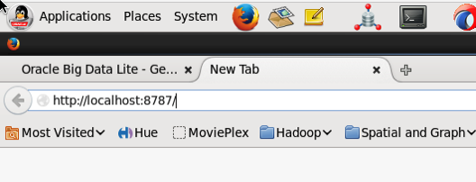
Open your favourite web browser and put in the host name or the IP address of your server. In my example I'm using the Oracle DB Developer VM to demonstrate the install, so I can use localhost, followed by the port number for RStudio Server.

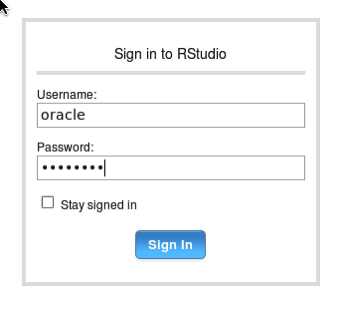
Log in using your Server username and password. This is oracle/oracle on the VM.

4. Use and Enjoy

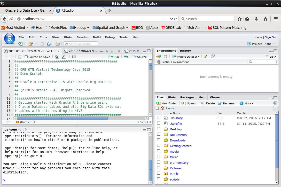
If you get logged into RStudio Server then you will see a screen something like the following!

Job Done and Enjoy!

5. An Extra Step is using the Oracle DB Developer VM

If you want to use RStudio on the Oracle DB Developer VM from your local OS, then you will need to open the port 8787 on the VM. To do this power down the VM, if you have it open. The open the Network section of the VM settings. I'm using VirtualBox. And then click on the Port Forwarding.

Click on OK to save your Port Forwarding setting and then click on the OK button again to close the Network settings for the VM.

Now start up the VM. When it has loaded and you have the desktop displayed in the VM window, you should now be able to connect to RStudio in the VM, from your local machine.

To do this open your web browser on your local machine and type in

http://localhost:8787

You should now get the RStudio login in screen that is shown in point 3 above. Go ahead, login and enjoy.

6. A little warning

Make sure to log out of RStudio when you are finished using it. If you don't then your R environment may not have been saved and you will get a message when you log in next. Now we don't want that happenings, so just log out of RStudio. You can do that by looking at the top right hand corner of the RStudio Server application.

I will have one more blog post on how you can configure RStudion Server to work with an Oracle Database server that has Oracle R Enterprise installed.

Installing RStudio Server on Oracle BigDataLite VM

A very popular tool for data scientists is RStudio. This tool allows you to interactively work with your R code, view the R console, the graphs and charts you create, manage the various objects and data frames you create, as well shaving easy access to the R help documentation. Basically it is a core everyday tool.

The typical approach is to have RStudio installed on your desktop or laptop. What this really means is that the data is pulled to your desktop or laptop and all analytics is performed there. In most cases this is fine but as your data volumes goes does does the limitations of using R on your local machine.

An alternative is to install a version called RStudio Server on an analytics server or on the database server. You can now use the computing capabilities of this server to overcome some of the limitations of using R or RStudio locally. Now you will use your web browser to access RStudio Server on your database server.

In this blog post I will walk you through how to install and get connected to RStudio Server on the Oracle BigDataLite VM.

After starting up the Oracle BigDataLite VM and logging into the Oracle user (password=welcome1) you will see the Start Here icon on the desktop. You will need to double click on this.

This will open a webpage on the VM that contains details of all the various tools that are installed on the VM or are ready for you to install and configure. This information contains all the http addresses and ports you need to access each of these tools via a web browser or some other way, along with the usernames and passwords you need to use them.

One of the tools lists is for RStudio Server. This product is not installed on the VM but Oracle has provided a script that you can run to perform the install in an automated way. This script is located in:

[oracle@bigdatalite ~]$ cd  /home/oracle/scripts/

Use the following command to run the RStudio Server install script.

[oracle@bigdatalite scripts]$ ./install_rstudio.sh

The following is the output from running this script and it will be displayed in your terminal window. You can use this to monitor the progress of the installation.

Retrieving RStudio
--2016-03-12 02:06:15--  https://download2.rstudio.org/rstudio-server-rhel-0.99.489-x86_64.rpm
Resolving download2.rstudio.org... 54.192.28.12, 54.192.28.54, 54.192.28.98, ...
Connecting to download2.rstudio.org|54.192.28.12|:443... connected.
HTTP request sent, awaiting response... 200 OK
Length: 34993428 (33M) [application/x-redhat-package-manager]
Saving to: `rstudio-server-rhel-0.99.489-x86_64.rpm'

100%[======================================>] 34,993,428  5.24M/s   in 10s     

2016-03-12 02:06:26 (3.35 MB/s) - `rstudio-server-rhel-0.99.489-x86_64.rpm' saved [34993428/34993428]

Installing RStudio
Loaded plugins: refresh-packagekit, security, ulninfo
Setting up Install Process
Examining rstudio-server-rhel-0.99.489-x86_64.rpm: rstudio-server-0.99.489-1.x86_64
Marking rstudio-server-rhel-0.99.489-x86_64.rpm to be installed
public_ol6_UEKR3_latest                                  | 1.2 kB     00:00     
public_ol6_UEKR3_latest/primary                          |  22 MB     00:03     
public_ol6_UEKR3_latest                                                 568/568
public_ol6_latest                                        | 1.4 kB     00:00     
public_ol6_latest/primary                                |  55 MB     00:12     
public_ol6_latest                                                   33328/33328
Resolving Dependencies
--> Running transaction check
---> Package rstudio-server.x86_64 0:0.99.489-1 will be installed
--> Finished Dependency Resolution

Dependencies Resolved

================================================================================
 Package        Arch   Version       Repository                            Size
================================================================================
Installing:
 rstudio-server x86_64 0.99.489-1    /rstudio-server-rhel-0.99.489-x86_64 251 M

Transaction Summary
================================================================================
Install       1 Package(s)

Total size: 251 M
Installed size: 251 M
Downloading Packages:
Running rpm_check_debug
Running Transaction Test
Transaction Test Succeeded
Running Transaction
  Installing : rstudio-server-0.99.489-1.x86_64                             1/1 
useradd: user 'rstudio-server' already exists
groupadd: group 'rstudio-server' already exists
rsession: no process killed
rstudio-server start/running, process 5037
  Verifying  : rstudio-server-0.99.489-1.x86_64                             1/1 

Installed:
  rstudio-server.x86_64 0:0.99.489-1                                            

Complete!
Restarting RStudio
rstudio-server stop/waiting
rsession: no process killed
rstudio-server start/running, process 5066

When the installation is finished you are now ready to connect to the RStudio Server. So open your web browser and enter the following into the address bar.

http://localhost:8787/

The initial screen you are presented with is a login screen. Enter your Linux username and password. In the case of the BigDataLite VM this will be oracle/welcome1.

Then you will be presented with the RStudio Server application in your web browser, as shown below. As you can see it is very similar to using RStudio on your desktop. Happy Days! You are now setup and able to run RStudio on the database server.

Make sure to log out of RStudio Server before closing down the window.

If you don't log out of RStudio Server then the next time you open RStudio Server your session will automatically open. Perhaps this is not the best for security, so try to remember to log out each time.

By now using RStudio Server on the Oracle Database server I can not get some of the benefits of computing capabilities of this server. Although there are still the typical limitations with of using R. But now I access RStudio on the database server and process the data on the database server, all from my local PC or laptop.

Everything is nicely setup and ready for you to install on the BigDataLite VM (thank you Oracle). But what about when we want to install RStudion Server on a different server. What are the steps necessary to install, configure and log in. Yes they should be similar but I will give a complete list of steps in my next blog post.

ORE video : Demo Code Part 2

The following is the second set of demo code from my video on using R in the Oracle Database. Check out the video before using the following code. The blog post for the video will be updated to contain links to all blog posts that have the various demo code.

The following code gives a very quick demonstration of using the RORACLE R package to access the data in your Oracle schema. ROracle has a number of advantages over using RJDBC and most of the advantages are about the performance improvements. Typically when using ROracle you will see a many fold improvement with selecting data and moving it to your R client, processing data in the database and also writing data back to the Oracle Database. In some tests you can see a 7 times improvement in performance over RJDBC. Now that is a big difference.

But the problem with ROracle is that it is only available on certain platforms/OS. For example it is not officially available for the Mac. But if you google this issue carefully you will find unofficial ways over coming this problem.

ROracle is dependent on Oracle Client. So you will need to have Oracle Client installed on you machine and have it available on the search path.

When you have Oracle Client installed and the ROracle R package installed you are ready to start using it.

So here is the demo code from the video.

> library(ROracle)
> drv <- dbDriver("Oracle")
> # Create the connection string
> host <- "localhost"
> port <- 1521
> sid <- "orcl"
>connect.string <- paste("(DESCRIPTION=”, "(ADDRESS=(PROTOCOL=tcp)(HOST=", host, ")(PORT=", port, "))",
>    "(CONNECT_DATA=(SID=", sid, ")))", sep = "")

> con <- dbConnect(drv, username = "dmuser", password = "dmuser",dbname=connect.string)

> rs <- dbSendQuery(con, "select view_name from user_views")
> # fetch records from the resultSet into a data.frame
> data <- fetch(rs)
> # extract all rows
> dim(data)
[1] 6 1
> data
                  VIEW_NAME
1       MINING_DATA_APPLY_V
2       MINING_DATA_BUILD_V
3        MINING_DATA_TEST_V
4  MINING_DATA_TEXT_APPLY_V
5  MINING_DATA_TEXT_BUILD_V
6   MINING_DATA_TEXT_TEST_V
> dbCommit(con)
> dbClearResult(rs)
> dbDisconnect(con)

ORE Video : Demo Code part 1

In a previous blog post I posted a video on using R with the Oracle Database and using Oracle R Enterprise. This is a part 1 extension of that blog post that gives the first set of demo code.

This first set of demonstration code is for using RJDBC to connect to the Oracle Database. Using RJDBC relies on using the JDBC jar file for Oracle. It is easily found in various installations of Oracle products and will be called something like ojdbc.jar. I like to take a copy of this file and place it in the root/home directory.

> library(RJDBC)
> # Create connection driver and open 
> connectionjdbcDriver <- JDBC(driverClass="oracle.jdbc.OracleDriver", classPath="c:/ojdbc6.jar")
> jdbcConnection <- dbConnect(jdbcDriver, "jdbc:oracle:thin:@//localhost:1521/orcl", "dmuser", "dmuser")
> #list the tables in the schema
> #dbListTables(jdbcConnection)
> #get the DB connections details - it get LOTS of info - Do not run unless it is really needed
> dbGetInfo(jdbcConnection)
> # Query on the Oracle instance name.
> #instanceName <- dbGetQuery(jdbcConnection, "SELECT instance_name FROM v$instance")
              TABLE_NAME1 
1  INSUR_CUST_LTV_SAMPLE2            
2              OUTPUT_1_2
> #print(instanceName)tableNames <- dbGetQuery(jdbcConnection, "SELECT table_name from user_tables where  
                                                 table_name not like 'DM$%' and table_name not like 'ODMR$%'")
> print(tableNames)
> viewNames <- dbGetQuery(jdbcConnection, "SELECT view_name from user_views")print(viewNames)
1       MINING_DATA_APPLY_V
2       MINING_DATA_BUILD_V
3        MINING_DATA_TEST_V
4  MINING_DATA_TEXT_APPLY_V
5  MINING_DATA_TEXT_BUILD_V
6   MINING_DATA_TEXT_TEST_V

> v <- dbReadTable(jdbcConnection, "MINING_DATA_BUILD_V")
> names(v)
[1] "CUST_ID"                 "CUST_GENDER"             "AGE"                     
[4] "CUST_MARITAL_STATUS"     "COUNTRY_NAME"            "CUST_INCOME_LEVEL"       
[7] "EDUCATION"               "OCCUPATION"              "HOUSEHOLD_SIZE"         
[10] "YRS_RESIDENCE"           "AFFINITY_CARD"           "BULK_PACK_DISKETTES"    
[13] "FLAT_PANEL_MONITOR"      "HOME_THEATER_PACKAGE"    "BOOKKEEPING_APPLICATION”
[16] "PRINTER_SUPPLIES"        "Y_BOX_GAMES"             "OS_DOC_SET_KANJI" 
> dim(v)
[1] 1500   18
> summary(v)
    CUST_ID       CUST_GENDER             AGE        CUST_MARITAL_STATUS COUNTRY_NAME       
Min.   :101501   Length:1500        Min.   :17.00   Length:1500         Length:1500        
1st Qu.:101876   Class :character   1st Qu.:28.00   Class :character    Class :character   
Median :102251   Mode  :character   Median :37.00   Mode  :character    Mode  :character   
Mean   :102251                      Mean   :38.89                                          
3rd Qu.:102625                      3rd Qu.:47.00                                          
Max.   :103000                      Max.   :90.00                                          
CUST_INCOME_LEVEL   EDUCATION          OCCUPATION        HOUSEHOLD_SIZE     YRS_RESIDENCE    
Length:1500        Length:1500        Length:1500        Length:1500        Min.   : 0.000   
Class :character   Class :character   Class :character   Class :character   1st Qu.: 3.000   
Mode  :character   Mode  :character   Mode  :character   Mode  :character   Median : 4.000                                                                               
                                                                            Mean   : 4.089                                                                               
                                                                            3rd Qu.: 5.000                                                                               
                                                                            Max.   :14.000 
> hist(v$RESIDENCE)
> hist(v$AGE)
> dbDisconnect(jdbcConnection)

Make sure to check out the other demonstration scripts that are shown in the video.

Oracle R Enterprise 1.5 (new release)

The Oracle Santa had a busy time just before Christmas with the release of several new version of products. One of these was Oracle R Enterprise version 1.5.

Oracle R Enterprise (1.5) is part of the Oracle Advanced Analytics option for the enterprise edition of the Oracle Database.

As with every new release of a product there are a range of bug fixes. But with ORE 1.5 there are also some important new features. These important new features include:

• New Random Forest specific for ORE.
• New ORE Data Store functions and privileges.
• Partitioning on multiple columns for ore.groupApply.
• Multiple improvements to ore.summary.
• Now performs parallel in-database execution for functions prcomp and svd.
• BLOB and CLOB data types are now supported in some of the ORE functions.

Check out the ORE 1.5 Release Notes for more details on the new features.

ORE 1.5 is only certified (for now) on R 3.2.x in both the open source version and the Oracle R Distribution version 3.2.

Check out the ORE 1.5 Documentation.

You can download ORE 1.5 Server side and Client side software here.