Wednesday, July 15, 2015

Charting Number of R Packages over time (Part 1)

This is the first of a three part blog post on charting and analysing the number of R package submissions.

(I will update this blog post with links to the other two posts as they come available)

I'm sure most of you have heard of the R programming language. If not then perhaps it is something that you might want to go off an learn a bit about. Why? well it is one of the most popular languages for performing various types of statistics, advanced topics on statistics and machine learning and for generating lots of cool looking graphs.

If this is not something that you might be interested then it is time to go to another website/blog.

In this blog post I'm going to chart the number of packages submitted to R and are available for download and installation.

Why am I doing this? I got bored one day after coming back from my vacation and I though it would be a useful thing to do. Then after doing this I decided to use these graphs somewhere else, but you will have to wait until 2016 to find out!

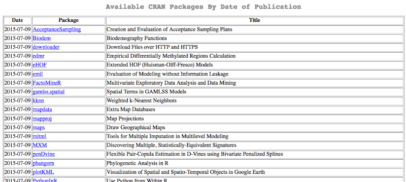
The R website has a listing of all the packages and the dates that they were submitted.
NewImage

There are a variety of tools available that you can use to extract the information on this webpage and there are lots of examples or R code too. I'll leave that as a little exercise for you to do.

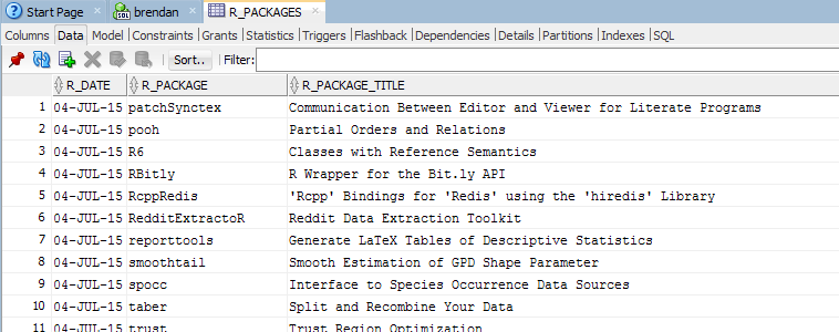
I extracted all of this information and stored it in a table in my Oracle Database (of course I did as I work with Oracle databases day in day out). This will allow me to easily reuse this data whenever I need it plus I can update this table with new packages from time to time.
NewImage

The following R code:

  1. Setups up and ROracle connection to my schema in my database
  2. Connects to the database
  3. Setups up a query to extract the data from the table
  4. Fetches this data into an R data frame called data
  5. Reformat the date columns to remove the time element to it
  6. Plot the data
library(ROracle)

drv <- dbDriver("Oracle")
# Create the connection string
host <- "localhost"
port <- 1521
service <- "pdb12c"
connect.string <- paste(
  "(DESCRIPTION=",
  "(ADDRESS=(PROTOCOL=tcp)(HOST=", host, ")(PORT=", port, "))",
  "(CONNECT_DATA=(SERVICE_NAME=", service, ")))", sep = "")

con <- dbConnect(drv, username = "brendan", password = "brendan",dbname=connect.string)

res<-dbSendQuery(con, "select r_date, count(*) r_num from r_packages
                       group by r_date order by 1 asc")
data <- fetch(res)

rdate<- data$R_DATE
rdate2<-as.Date(rdate,"%d/%m/%y")

plot(data$R_NUM~rdate2, data, type="l" , xaxt="n")
axis(1, rdate2, format(rdate2, "%b %y"), cex.axis=.7, las=1)

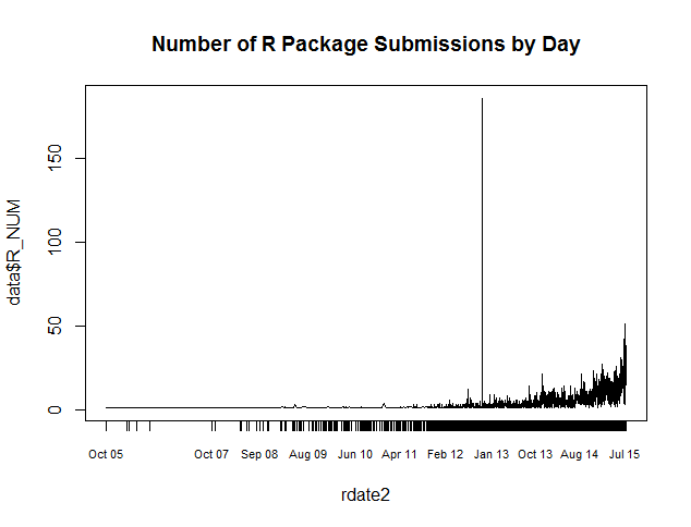
After I run the above code I get the following plot.
NewImage

(Yes I could have done a better job on laying out the chart with all sorts of labels and colors etc)

This chart gives us a plot of the number of new submissions by day.

There are 2 very obvious things that stand out from this graph. The easiest one to deal with is that we can see that there has been substantical growth in new submissions over the past 3 years. Perhaps we need to examine these a bit closer and when you do you will find that a lot of these are existing packages that have been resubmitted with updates.

There is a very obvious peak just over half ways along the chart. We really need to investigate this to understand what has happended. This peak occurs on the 29th October 2012. What happened on the 29th October 2012 as this is clearly an anomaly with the rest of the data. Well on this date R version 2.15.2 was release and a there was a lot of update pagackes got resubmitted.

Check out my next two blog posts were I will explore this data in a bit more detail.
Part 2 blog post

Part 3 blog post

Monday, July 13, 2015

V506 of Oracle OBIEE SampleApp Virtual Machine

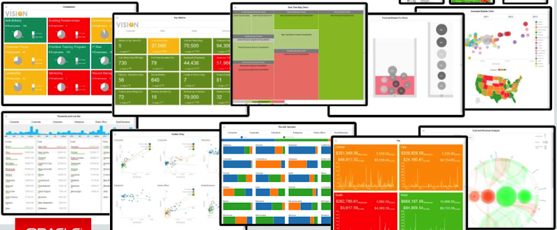
A few days ago Oracle released the latest version of the Virtual Machine for OBIEE SampleApp. The current version has a number of new features and new product versions (see below).

To get this latest version go to the following link to download the VM files and to install. As always this is a beast of a VM and you should only consider the install and setup if you have the space and in particular you have 16G RAM.

Oracle Business Intelligence Enterprise Edition Samples on OTN.

NewImage

v506 New Features

  • DB 12.1.0.2 with the In-Memory option
  • Load and process JSON data
  • Integrates with Big Data SQL
  • Connects to Impala
  • Session tracking in UT
  • Exalytics Aggregation Functions
  • Lots of new Visualizations
  • Custom Style Features
  • Hierarchical Session Variables
  • etc.

Software on V506

  • Oracle Enterprise Linux 6.5 x64
  • OBIEE 11.1.1.9GA two distinct OBIEE instances, Essbase 11.1.2.4, updated BIMAD
  • Oracle MapViewer11.1.1.9.1
  • Oracle BICS Data Sync v1
  • Oracle Database 12c IMDB 12.1.0.2, PDB Install, AWM 12.1.0.2a, APEX 4.2.6 & ORDS 2.0.1, ODM, Oracle Spatial and Graph
  • ORE 1.4.1 & R 3.1.1
  • ENDECA 3.1, Server 7.6.1, Studio 3.1, Provisioning Services
  • Cloudera CDH 5.1.2, Oracle BigData SQL, Oracle BigData Connectors
  • Plug and Play Companions : EPM 11.1.2.3, BIApps Demos
  • Utils: Start scripts, MapBuilder, SQLDev 4.1
NewImage

Thursday, July 9, 2015

Oracle Architect's Guides to Big Data

Over the past couple of years we have had a lot of information about Big Data presented to us. But one of the things that still stands out is that there is still a bit of confusion on what Big Data is. Depending on who you are talking to you will get a different definition and interpretation of what Big Data is and what you can do with it.

For example there is one company I know of who are talking about their Big Data project. For them this involves processing approx. 1 million records. That is Big for them. For others that is tiny.

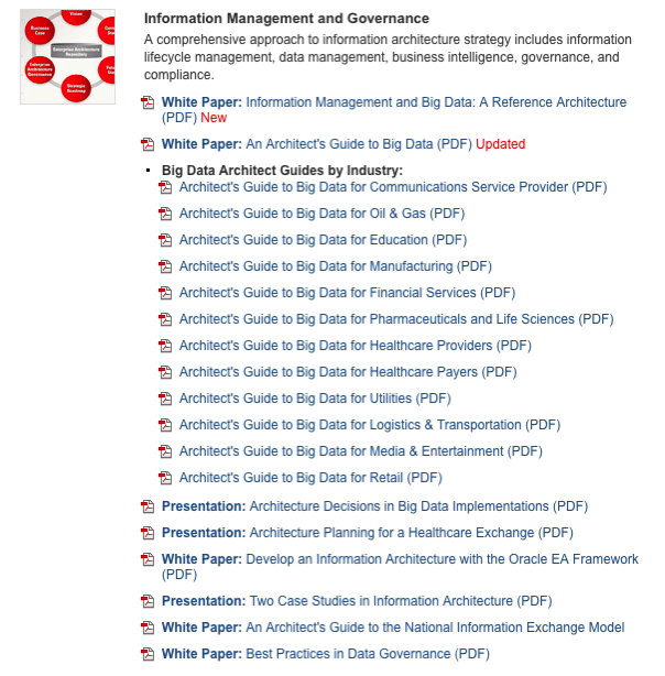
Oracle has recently put together a series of articles that talk about what architectural changes are needed to your technical infrastructure to support Big Data. In this case it is more about the volume of data rather than different types of data. Although this is covered by the architecture that Oracle gives.

As part of the Oracle Enterprise Architecture section of the Oracle website, they have put together a series of articles on how you can include Big Data within your Enterprise Information Architecture.

These are a good read and a great place to get a better understanding of what you need to be considering as you move to an architecture that includes Big Data.

NewImage

Wednesday, July 1, 2015

Extending vmdk Size for VirtualBox VM

Recently I ran out of space on one of my Windows virtual machines. I needed to increase the size of the disk to allow me to install some new software. When creating the VM I had created the disks as VMDK. Yes I know now that is not the best format to use :-( VMDK disks/files do not allow you to dynamically change their size :-( So what can you do? Is it possible in any way? If so how? Well this is what I did (after a bit of research using the google and StackOverFlow.
  1. Make a copy of the vmdk file on the OS. Just in case anything happens! (always have a backup)
  2. Clone the vmdk disk file into vdi format. To do this you need to use the VBoxManage command/app to clone the file into a vdi formatted file. For example this is what I ran.

    VBoxManage clonehd "Win7-11.2.0.3-ORE-03-Jan-14-disk1.vmdk" "cloned.vdi" --format vdi

  3. There was some suggestions that you could then clone the vdi file back into vmdk format. This did not work for me. It kept on giving me errors when the cloning process was nearly finished. After a bit of time researching this I wasn't able to find a solution to fix this. Instead I did the following
  4. Replace the vodka disk/file with the vdi disk/file in my VirtualBox VM. Open VirtualBox, select the VM and then click on the Storage section. In this I was able to add the new vdi disk/file and then removed the old vodka disk/file.

    NewImage

  5. Start up the VM. The VM starts up as normal and everything works OK.
  6. To allocate and make the extract space useable you need to allocated the new space to the c:\ drive. To do this I did the following:
  7. Click on Start Button, then right click on Computer and select Manage from the drop down menu.
  8. In the Computer Management console select Disk Management. A screen something like the following appears shows the amount of allocated and unallocated disk.

    NewImage

  9. Right click on the area for the c:\ drive and select Extend Volume from the drop down menu.
  10. Select all the defaults are you go through the Wizard to Extend the Volume. When you are finished the c:\ drive will be extended with all the extra space, as shown below.

    NewImage

  11. All done. You now have a larger disk/drive for your Windows VM.

Tuesday, June 23, 2015

Oracle Magazine - March/April 2001

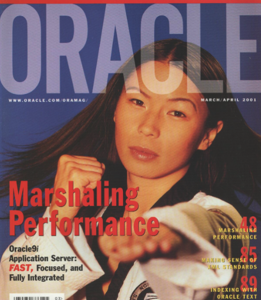
The headline articles of Oracle Magazine for March/April 2001 were on using Oracle 9i Application server to deliver e-business and web based applications. There was some case studies of companies using this technologies including Tantalus Communications, Digital River Commerce System, Tomatoland.com and Oracle themselves.


OM 2001 March April

Other articles included:

  • Tom Kyte's column looked at tips on automation, cleanup and database maintenance. Some of the details included index rebuilds, indexing interMedia files, killing and cleaning up sessions, how to specify the column at runtime in an order by, and how to use DBMS_JOB for database maintenance.
  • Oracle announces the release of PORTAL.ORACLE.COM and MY.ORACLE.COM.
  • Fre Sansmark has an article on Database Benchmarking and discusses what it means and how well they address real-world performance questions.
  • Understanding XML Standards gives a brief introduction to what XML is about, explains the three layers of XML Grammar, XML based Protocols and XML Vocabularies. .
  • Part 3 of 'Exploring Oracle Text Basics' looks at text searching and comparisons, creating, indexing and loading data.
  • Creating Updatable Views explores the various requirements for creating an View that can be used to update data that is based on a single table or based on the joining of multiple tables..
  • Linking to Remote Databases explores the basics of Database Links and that the DBA needs to know to setup and manages these..
  • Steven Feuerstein's article looks at Advanced Native Dynamic SQL and the use of bind variables and their limitations.

To view the cover page and the table of contents click on the image at the top of this post or click here.

My Oracle Magazine Collection can be found here. You will find links to my blog posts on previous editions and a PDF for the very first Oracle Magazine from June 1987.

Monday, June 8, 2015

Blogger vs WordPress Evaluation

I have my blog (come website) on the go for a few years now. It all started out as a notebook really for myself and a way of recording certain things so that I could find them easily later.
Over time it has developed into some more that that and it now covers a number of technical how-to type of articles and some of my Oracle User Group (and ACE Director) activities.
It all started out on Blogger that is provided by Google. I've found Blogger really easy to use and to configure into getting something that is semi professional looking (at least it does to me).
All of this happened before WordPress really got going. I've had a look at WordPress from time to time over the years but never really invested enough time into it. Despite, what feels like everyone, saying that WordPress was the bees knees.
About 6 weeks ago I decided to put some solid time into investigating WordPress (about time some of you might say). The challenge for me was how easy would it be to replicate what I had on my blogger hosted website onto WordPress. I have to say it was easy enough.
Now I have 2 blogs / website running in parallel. Currently my blog/website is hosted on Blogger can it can be accessed via my custom domain of www.oralytics.com. The WordPress blog/website can be accessed at oralytics.wordpress.com
As you will see they are very similar to each other. Yes there are some cosmetic differences but all the content is the same.
What I'm going to do is to run these two environments in parallel for the next (maybe) 6 to 8 weeks. At some point I will switch over my domain name (www.oralytics.com) to point at the WordPress site. And then I might switch it back.
The big question for me to answer is to which one of these 2 environments will become my main site.
Blogger is FREE.
WordPress is FREE, well it is if I use the WordPress.com site.
But if I use the WordPress.com site then I get this annoying banner at the bottom of the browser window that does some advertising for WordPress and the Theme that I'm using.
The alternative to this where I do not get any of these adverts appearing is to pay for Hosting and to pay for a theme. Over a 3 year period that comes out at about $300+. The cheapest WordPress hosting that I could find, at the moment, is with GoDaddy.
What do you think I should do?
1. Stay with what I have on Blogger (www.oralytics.com) (Free)
2. Switch to the Free WordPress.com option (oralytics.wordpress.com) (Free)
3. Buy WordPress hosting and pay for a theme. (Costs $)
When I put out my original enquiry a few weeks ago lots of people came back with really good advice. In particular I wanted to mention Jeff Smyth, Tim Hall and Martin Widlake for the advice, help and suggestions, which I think lots of others found very useful.

Wednesday, June 3, 2015

PMML in Oracle Data Mining

PMML (Predictive Model Markup Langauge) is an XML formatted output that defines the core elements and settings for your Predictive Models. This XML formatted output can be used to migrate your models from one data mining or predictive modelling tool to another data mining or predictive modelling tool, such as Oracle.

Using PMML to migrate your models from one tool to another allows for you to use the most appropriate tools for developing your models and then allows them to be imported into another tool that will be used for deploying your predictive models in batch or real-time mode. In particular the ability to use your Predictive Model within your everyday applications enables you to work in the area of Automatic or Prescriptive Analytics. Oracle Data Mining and the Oracle Database are ideal or even the best possible tools to allow for Automatic and Prescriptive Analytics for your transa

PMML is an XML based standard specified by the Data Mining Group

Oracle Data Mining supports the importing of PMML models that are compliant with version 3.1 of the standard and for Regression Models only. The regression models can be for linear regression or binary logistic regression.

The Data Mining Group Archive webpage have a number of sample PMML files for you to download and then to load into your Oracle database.

To Load the PMML file into your Oracle Database you can use the DBMS_DATA_MINING.IMPORT_MODEL function. I’ve given examples of how you can use this function to import an Oracle Data Mining model that was exported using the EXPORT_MODEL function.

The syntax of the IMPORT_MODEL function when importing a PMML file is the following

DBMS_DATA_MINING.IMPORT_MODEL (
      model_name        IN  VARCHAR2,
      pmmldoc           IN  XMLTYPE
      strict_check      IN  BOOLEAN DEFAULT FALSE);

The following example shows how you can load the version 3.1 Logistic Regression PMML file from the Data Mining Group archive webpage

NewImage


BEGIN    
   dbms_data_mining.IMPORT_MODEL (‘PMML_MODEL',
        XMLType (bfilename (‘IMPORT_DIR', 'sas_3.1_iris_logistic_reg.xml'),
          nls_charset_id ('AL32UTF8')
        ));
END;


This example uses the default value for STRICT_CHECK as FALASE. In this case if there are any errors in the PMML structure then these will be ignored and the imported model may contain “features” that may make it perform in a slightly odd manner.

Wednesday, May 27, 2015

R (ROracle) and Oracle DATE formats

 When you comes to working with R to access and process your data there are a number of little features and behaviours you need to look out for.

One of these is the DATE datatype.

The main issue that you have to look for is the TIMEZONE conversion that happens then you extract the data from the database into your R environment.

There is a datatype conversions from the Oracle DATE into the POSIXct format. The POSIXct datatype also includes the timezone. But the Oracle DATE datatype does not have a Timezone part of it.

When you look into this a bit more you will see that the main issue is what Timezone your R session has. By default your R session will inherit the OS session timezone. For me here in Ireland we have the time timezone as the UK. You would time that the timezone would therefore be GMT. But this is not the case. What we have for timezone is BST (or British Standard Time) and this takes into account the day light savings time. So on the 26th May, BST is one hour ahead of GMT.

OK. Let's have a look at a sample scenario.

The Problem

As mentioned above, when I select date of type DATE from Oracle into R, using ROracle, I end up getting a different date value than what was in the database. Similarly when I process and store the data.

The following outlines the data setup and some of the R code that was used to generate the issue/problem.

Data Set-up
Create a table that contains a DATE field and insert some records.

CREATE TABLE STAFF
    (STAFF_NUMBER VARCHAR2(20),
       FIRST_NAME VARCHAR2(20),
       SURNAME VARCHAR2(20),
       DOB DATE,
       PROG_CODE VARCHAR2(6 BYTE),
       PRIMARY KEY (STAFF_NUMBER));

insert into staff values (123456789, 'Brendan', 'Tierney', to_date('01/06/1975', 'DD/MM/YYYY'), 'DEPT_1');
insert into staff values (234567890, 'Sean', 'Reilly', to_date('21/10/1980', 'DD/MM/YYYY'), 'DEPT_2');
insert into staff values (345678901, 'John', 'Smith', to_date('12/03/1973', 'DD/MM/YYYY'), 'DEPT_3');
insert into staff values (456789012, 'Barry', 'Connolly', to_date('25/01/1970', 'DD/MM/YYYY'), 'DEPT_4');


You can query this data in SQL without any problems. As you can see there is no timezone element to these dates.

Selecting the data
I now establish my connection to my schema in my 12c database using ROracle. I won't bore you with the details here of how to do it but check out point 3 on this post for some details.

When I select the data I get the following.

> res<-dbsendquery br="" con="" from="" select="" staff="">> data <- br="" fetch="" res="">> data$DOB
[1] "1975-06-01 01:00:00 BST" "1980-10-21 01:00:00 BST" "1973-03-12 00:00:00 BST"
[4] "1970-01-25 01:00:00 BST"


As you can see two things have happened to my date data when it has been extracted from Oracle. Firstly it has assigned a timezone to the data, even though there was no timezone part of the original data. Secondly it has performed some sort of timezone conversion to from GMT to BST. The difference between GMT and BTS is the day light savings time. Hence the 01:00:00 being added to the time element that was extract. This time should have been 00:00:00. You can see we have a mixture of times!

So there appears to be some difference between the R date or timezone to what is being used in Oracle.

To add to this problem I was playing around with some dates and different records. I kept on getting this scenario but I also got the following, where we have a mixture of GMT and BST times and timezones. I'm not sure why we would get this mixture.

> data$DOB
[1] "1995-01-19 00:00:00 GMT" "1965-06-20 01:00:00 BST" "1973-10-20 01:00:00 BST"
[4] "2000-12-28 00:00:00 GMT"


This is all a bit confusing and annoying. So let us look at how you can now fix this.

The Solution
Fixing the problem : Setting Session variablesWhat you have to do to fix this and to ensure that there is consistency between that is in Oracle and what is read out and converted into R (POSIXct) format, you need to define two R session variables. These session variables are used to ensure the consistency in the date and time conversions.

These session variables are TZ for the R session timezone setting and Oracle ORA_SDTZ setting for specifying the timezone to be used for your Oracle connections.

The trick there is that these session variables need to be set before you create your ROracle connection. The following is the R code to set these session variables.

> Sys.setenv(TZ = "GMT")
> Sys.setenv(ORA_SDTZ = "GMT")

So you really need to have some knowledge of what kind of Dates you are working with in the database and if a timezone if part of it or is important. Alternatively you could set the above variables to UDT.

Selecting the data (correctly this time)
Now when we select our data from our table in our schema we now get the following, after reconnecting or creating a new connection to your Oracle schema.

> data$DOB
[1] "1975-06-01 GMT" "1980-10-21 GMT" "1973-03-12 GMT" "1970-01-25 GMT"
Now you can see we do not have any time element to the dates and this is correct in this example. So all is good.

We can now update the data and do whatever processing we want with the data in our R script.

But what happens when we save the data back to our Oracle schema. In the following R code we will add 2 days to the DOB attribute and then create a new table in our schema to save the updated data.

> data$DOB
[1] "1975-06-01 GMT" "1980-10-21 GMT" "1973-03-12 GMT" "1970-01-25 GMT"

> data$DOB <- br="" data="" days="">> data$DOB
[1] "1975-06-03 GMT" "1980-10-23 GMT" "1973-03-14 GMT" "1970-01-27 GMT"


> dbWriteTable(con, "STAFF_2", data, overwrite = TRUE, row.names = FALSE)
[1] TRUE


I've used the R package Libridate to do the date and time processing.

When we look at this newly created table in our Oracle schema we will see that we don't have DATA datatype for DOB, but instead it is created using a TIMESTAMP data type.


If you are working with TIMESTAMP etc type of data types (i.e. data types that have a timezone element that is part of it) then that is a slightly different problem. Perhaps one that I'll look at soonish.

Thursday, May 14, 2015

Extracting Oracle data & Generating JSON data file using ROracle

In a previous blog post I showed you how to take a JSON data file and to load it into your Oracle Schema using R. To do this I used ROracle to connect to the database and jsonlite to do the JSON processing of the data.
Alternatives to using ROracle would be RODBC, RJDBC and DBI. So you could use one of these to connect to the database.
In this post I want to show you how to extract data from an Oracle table (or view) and to output it to a file in JSON format. Again I will be using the jsonlite R package to perform all the JSON formatting work for me.
1. Connect to the Database
This is the same connect setup that I used in the previous post.
# initialise the packages
> library(ROracle)
> library(jsonlite)
# Create the connection string
> drv <- dbdriver="" p="" racle="">
> host <- localhost="" p="">
> port <- 1521="" p="">
> service <- p="" pdb12c="">
> connect.string <- p="" paste="">
"(DESCRIPTION=",
"(ADDRESS=(PROTOCOL=tcp)(HOST=", host, ")(PORT=", port, "))",
"(CONNECT_DATA=(SERVICE_NAME=", service, ")))", sep = "")
# establish the connection
> con <- dbconnect="" dbname="connect.string)" drv="" p="" password="dmuser" username="dmuser">


2. Read the data from the table/view
Read the data from the table into a R data frame.
> rs <- con="" dbsendquery="" from="" mining_data_build_v="" p="" select="">
> data <- fetch="" p="" rs="">
> dim(data)
[1] 1500 18
> head(data, 3)
CUST_ID CUST_GENDER AGE CUST_MARITAL_STATUS COUNTRY_NAME
1 101501 F 41 NeverM United States of America
2 101502 M 27 NeverM United States of America
3 101503 F 20 NeverM United States of America
CUST_INCOME_LEVEL EDUCATION OCCUPATION HOUSEHOLD_SIZE YRS_RESIDENCE AFFINITY_CARD
1 J: 190,000 - 249,999 Masters Prof. 2 4 0
2 I: 170,000 - 189,999 Bach. Sales 2 3 0
3 H: 150,000 - 169,999 HS-grad Cleric. 2 2 0
BULK_PACK_DISKETTES FLAT_PANEL_MONITOR HOME_THEATER_PACKAGE BOOKKEEPING_APPLICATION
1 1 1 1 1
2 1 1 0 1
3 1 0 0 1
PRINTER_SUPPLIES Y_BOX_GAMES OS_DOC_SET_KANJI
1 1 0 0
2 1 1 0
3 1 1 0


We now have the data from the table in a data frame called data. We can now use this data frame to covert the data into JSON.
3. Convert into JSON format
To produced the JSON formatted output of the data in our table (or view) we can use the toJSON function that produces the outputted JSON data in an R String.
> jsonData <- data="" p="" tojson="">
> jsonData

4. Create the JSON file
We are now ready to output the formatted JSON data out to file. We can use the R function 'write' to write the JSON data out to a file.
> write(jsonData, file="c:/app/demo_json_data2.json")
Job Done!
5. Verify the JSON data was created correctly
To verify that JSON data file was created correctly, we can use the steps outlined in my previous post to read in the file. If all the correct then we should get no errors.
> jsonFile <- app="" c:="" demo_json_data2.json="" p="">
> jsonData <- fromjson="" jsonfile="" p="">
> str(jsonData)
> names(jsonData)
> nrow(jsonData)


You will notice that there is one difference between the code shown above and what I showed in my previous example/blog post. This time we don't have an extra wrapper class of Items.
Generating JSON data - Using SQL Developer
In my previous post I showed you one way of generating a JSON file based on the data in a table. You could do that using SQL Developer and SQLcl.
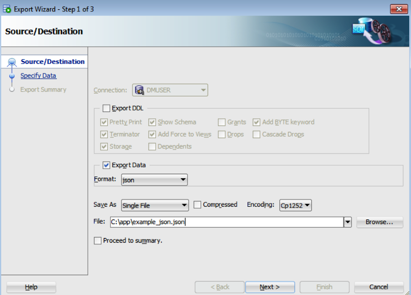
An alternative is to use the Table Export feature to export the data in JSON format.
To do this right click on the table (or view) and select Export from the drop down menu.
The Export Wizard will open. De-select the Export DDL tick box. In the export data section change the format drop-down to JSON. Then enter the location and file name for the JSON file. Then click the next buttons until you are finished.
Blog json

Friday, May 8, 2015

Loading JSON data into Oracle using ROracle and jsonlite

In this post I want to show you one way of taking a JSON file of data and loading it into your Oracle schema using ROracle. The JSON data will then be used to create a table in your schema. Yes you could use other methods to connect to the database and to create the table. But ROracle is by far the fastest method of connecting, selecting and processing data.

1. Necessary R Packages

You will need two R library. The first of these is the ROracle package. This gives us all the connection and data processing commands to work with the Oracle database. The second package is the jsonlite R package. This package allows us to open, read and process a file that has JSON data.

> install.package("ROracle")

> install.package("jsonlite")

After you have installed the packages you can now load them into your R environment so that you can use them in your current session.

> library(ROracle)

> library(jsonlite)

Depending on your version of R you may get some working messages about the libraries being built under a different version of R. Then again maybe you won't get these :-)

2. Open & Read the JSON file in R

Now you are ready to name and open the file that contains your JSON data. In my case the file is called 'demo_json_data.json'

> jsonFile <- "c:/app/demo_json_data.json"

> jsonData <- fromJSON(jsonFile)

We now have the JSON data loaded into R. We can now look at the attributes of each JSON record and the number of records that was in the JSON file.

> names(jsonData$items)

[1] "cust_id" "cust_gender" "age"

[4] "cust_marital_status" "country_name" "cust_income_level"

[7] "education" "occupation" "household_size"

[10] "yrs_residence" "affinity_card" "bulk_pack_diskettes"

[13] "flat_panel_monitor" "home_theater_package" "bookkeeping_application"

[16] "printer_supplies" "y_box_games" "os_doc_set_kanji"

> nrow(jsonData$items)

[1] 1500

As you can see the records are grouped under a higher label of 'items'. You might want to extract these records into a new data frame.

> data <- jsonData$items

>

Now we have our data ready in a data frame and we can use this data frame to create a table and insert the data.

3. Create the connection to the Oracle Schema

I have a previous post on connecting to an Oracle Schema using ROracle. That was connecting to an 11g Oracle Database.

JSON is a new feature in Oracle 12c and the connection details are a little bit different because we are now having to deal with connection to a pluggable database. The following illustrates connecting to a 12c database and assumes you have Oracle Client already installed and configured with your tnsnames.ora entry.

# Create the connection string

> host <- "localhost"

> port <- 1521

> service <- "pdb12c"

> connect.string <- paste(

"(DESCRIPTION=",

"(ADDRESS=(PROTOCOL=tcp)(HOST=", host, ")(PORT=", port, "))",

"(CONNECT_DATA=(SERVICE_NAME=", service, ")))", sep = "")

> con2 <- dbConnect(drv, username = "dmuser", password = "dmuser",dbname=connect.string)

>

4. Create the table in your Oracle Schema

At this point we have our connection to our Oracle Schema setup and connected, we have read in the JSON file and we have the JSON data in a data frame. We are now ready to push the JSON data to a table in our schema.

> dbWriteTable(con, "JSON_DATA", overwrite=TRUE, value=data)

Job done :-)

The table JSON_DATA has been created and the data is stored in the table in typical table attributes and rows format.

One thing to watch our for with the above command is with the overwrite=TRUE parameter setting. This replaces a table if it already exists. So your old data will be gone. Be careful.

5. View and Query the data using SQL

When you now log into your schema in the 12c Database, you can now query the data in the JSON_DATA table. (Yes I know it is not in JSON format in this table).

NewImage

How did I get/generate my JSON data?

I generated the JSON file using a table that I already had in one of my schemas. This table is part of the sample data set that is built on top of the Oracle sample schemas.

The image below shows the steps involved in generating the data in JSON format. I used SQL Developer and set the SQLFORMAT to be JSON. I then ran the query to select the data. You will need to run this as a script. Then copy the JSON data and paste it into a file.

NewImage

The SQL FORMAT command sets the output format for a query back to the default query output format that we are well use to.

A nice little JSON viewer can be found at http://jsonviewer.stack.hu/

Copy and paste your JSON data into this and you can view the structure of the data. Check it out.

Monday, May 4, 2015

Oracle Data Miner (ODM 4.1) New Features

With the release of SQL Developer 4.1 we also get a number of new features with Oracle Data Miner (ODMr). These include:

  • Data Source node can now include data sources that contain JSON data, generating JSON schema and has a JSON viewer
  • Create Table can now create data in JSON
  • JSON Query Node allows you to view, query and process JSON data, combine it with relational data, generate sub-group by, and nested columns to be part of input to algorithms
  • New PL/SQL APIs for managing Data Miner projects and workflows. This includes run, cancel, rename, delete, import and export of workflows using PL/SQL.
  • New ODMr Repository views that allows us to query and monitor our workflows.
  • Transformation Node now allows you different ways of handling NULLS.
  • Transformation Node now allows us to create Custom Bins, define bin labels and bin values
  • Overall Workflow and ODMr environment improvements to allow for greater efficiency in workflow behaviour and interactions with the database. So using ODMr should feel quicker and more responsive.

What out for the Gotchas: Although support for JSON has been added to ODMr, as outlined above, you are still a bit limited to what else you can do with your JSON data. Based on the documentation you can use JSON data in the Association and Classification build nodes.

I'm not sure about the other nodes and this will need a bit of investigation to see what nodes can and cannot use JSON data. I'm sure this will all be sorted out in the next release.

Keep an eye out for some blog posts over the coming weeks on how to explore and use these new features of Oracle Data Miner.

SQL Developer 4.1 : ODM Repository upgrade

Earlier today (4th May) SQL Developer 4.1 was released :-)

For those of you who use the Oracle Data Miner tool (that is part of SQL Developer) you will need to upgrade your repository. The following steps will walk you through the process.

1. Download SQL Developer  (you do need to have Java 8 installed) This download does not come with the JRE built into it. This usually comes a few days after the release.

2. Unzip the downloaded file and copy the extracted directory to where you like to keep your applications etc.

3. Start up SQL Developer by running the sqldeveloper.exe file. This will located in the extracted folder  \sqldeveloper-4.1.0.19.07-no-jre\sqldeveloper

4. If you have been a previous install of SQL Developer you will be asked if you want to migrate your current settings. Click on the Yes button and all your connections and settings will be migrated.

Blog odm4 1 1

5. To upgrade your Oracle Data Miner (ODMr) repository, you will need to open one of your ODMr connections. When you do this ODMr will check to see if the repository in your database needs to be updated. If it does you will get the following window.

NewImage

6. Enter the password for SYS

NewImage

6. When you get the following window you can click on the Start button to begin the Oracle Data Miner repository upgrade.

NewImage

NewImage

7. After a couple of minutes (and depending on the number of ODM Workflows and ODM schemas to have) you will get the following window.

NewImage

Congratulations. You have now upgraded your Oracle Data Miner repository.

If you do encounter any errors during the upgrade of the repository then you should get onto the OTN Forum for Oracle Data Miner and report the errors. The Oracle Data Miner team monitor this forum and will get back to you quickly with a response.