Friday, October 30, 2015

My OOW15 is now over

It seems to be traditional for people to write a blog post that summaries their Oracle Open World (OOW) experience. Well here is my attempt and it really only touches on a fraction of what I did at OOW, which was one of busiest OOWs I've experienced.

It all began back on Wednesday 21st October when I began my journey. Yes that is 9 days ago, a long long 9 days ago. I will be glad to get to home.

The first 2 days here in San Francisco was down at Oracle HQ were the traditional Oracle ACE Directors briefings are held. I'm one of the small (but growing) number of ACEDs and it is an honour he take part in the programme. The ACE Director briefings are 2 days of packed (did I say they are packed) full on talks by the leading VPs, SVPs, EVPs and especially Thomas Kurian. Yes we had Thomas Kurian come into talk to us for 60-90 minutes of pure gold. We get told all the things that Oracle is going to release or announce at OOW and for the next few months and beyond. Some of things that I was particularly interested in was the 12.2 database stuff.

Unfortunately we are under NDA for all of the stuff we were told, until Oracle announce it themselves.

On the Thursday night a few of us meet up with Bryn Llewellyn (the god father of PL/SQL) for a meal. Here is a photo to prove it. It was a lively dinner with some "interesting" discussions.

NewImage

On the Friday we all transferred hotels into a hotel beside Union Square.

We had the Saturday free, and I'm struggling to remember what I actually did. But it did consist of going out and about around San Francisco. Later that evening there was a meet up arranged by "That" Jeff Smyth in a local bar.

Sunday began with me walking across (and back) the Golden Gate Bridge with a few other ACEDs and ACEs.

NewImage

The rest of the Sunday was spent at the User Groups Forum. I was giving 2 presentations. The first presentation was part of the "Another 12 things about Oracle 12c". For this session there was 15 presenters and we each had 7 minutes to talk about a topic. Mine was on Oracle R Enterprise. It was an almost full room, which was great.

NewImage NewImage

Then I had my second presentation right afterwards and for that we had a full room. I was co-presenting with Tony Heljula and we were talking about some of the projects we have done using Oracle Advanced Analytics.

NewImage

After that my conference duties were done and I got to enjoy the rest of the conference.

Monday and Tuesday were a bit mental for me. I was basically in sessions from 8am until 6pm without a break. There was lots of really good topics, but unfortunately there was a couple presentations that were total rubbish. Where the title and abstract had no relevance to what was covered in the presentation, and even the presentation was rubbish. There was only a couple of these.

Wednesday was the same as Monday and Tuesday but this time I had time for lunch.

As usual the evenings are taken up with lots of socials and although I had great plans to go to lots of them, I failed and only got to one or two each evening.

On Wednesday night we ended up out at Treasure Island to be entertained by Elton John and Becks, and then back into Union Square for another social.

Thursday was very quiet and as things started to wind down at OOW finishing up at 3pm. A few of us went down to Fishermans Wharf and Pier39 for a wander around and a meal. Here are the some photos from the restaurant.

NewImage NewImage

Friday has finally arrived and it is time to go home. OTN are very generous and put on a limo for the ACEDs to bring us out to the airport.

NewImage

As always there are lots of people to thank but I won't start naming names here as I'm sure I will forget someone. But I do want to thank all the gang in OTN that look after the Oracle ACE programme. You really look after us, not just at OOW, but all year round. It is with your support that I get to go to wonderful conferences and to OOW.

Wednesday, October 21, 2015

People from Ireland who are Speaking at #OOW15

Oracle Open World 2015 will be kicking off in a few days time. There will be over 50K people attending this event, with a couple of hundred speakers.

I'm one of the lucky ones to have been selected to speak at Oracle Open World. This will be my third or fourth year in a row that I'm speaking at Oracle Open World.

Am I the only person from Ireland who is speaking at Oracle Open World ? No, I'm not, but there is a small number of us this year. There are basically 2, yes 2 other people from Ireland speaking at Oracle Open World. These are Richard Corbridge from the HSE, and Debra Lilley.

If you are interesting in attending these sessions here is the schedule.

NewImage

Please share this information to allow your colleagues and help spread the news about he Irish Speakers.

If you are attending OOW, then please tweet, blog, Facebook, etc about these presentations.

Hopefully I will see you are one or both of my presentations on the Sunday.

And I will be having a draw/raffle for a copy of my book at my second presentation on the Sunday at 15:30 in Moscone South - 307

NewImage

Monday, October 19, 2015

My schedule for OOW15

It seems to be a things that people blog about their schedule for Oracle Open World and talk about how busy they will be.

So to join the club this is my current schedule.

NewImage

The boxes that are (a kind of) orange with red text are when I have MY presentations.

The purple boxes indicate some fun event and entertainment.

When attending conferences sometime you get to hear about a good presentation or some other events just happen. So this schedule is tentative and will probably only reflect 40%-60% of what I will really attend/do. There is so much going on each day.

You will see I have some Hands-on-Labs booked. These are a great way to try out some product for an hour. I highly recommend you doing some too.

By far my favourite part of my OOW trip is the Oracle ACE Director briefing that OTN arranges for us. This briefing will happen on the Thursday (22nd) and Friday (23rd) before OOW, and this is held in Oracle HQ in Redwood Shores.

We have been given a tentative schedule for the ACED Briefing and for me I highlight of this briefing is when Thomas Kurian comes in an very openly talks to us, telling us lots and lots and lots about what is happening across the Oracle product set. I would lover to be able to share what we are told but we are all under NDA. After Thomas we have some Cloud updates, then we get onto some updates on Oracle Development Tools, lots of updates on what is coming next in the Oracle Database. So we get the likes of Penny Avril, Andy Mendelsohn, Tom Michelini, Steven Feurerstein, Roland Smart and Wim Coekaerts, among others. So lots and lots of EVPs, Sr VPs and VPs.

After the briefing is over we then hop on a bus and head to our hotel in download San Francisco, near Union Square, where we will be based for the OOW.

Thanks to all in OTN and to those who run the Oracle ACE programme for arranging and paying for my flights, hotels and transportation.

Monday, October 12, 2015

SQL and PL/SQL icons and stickers

Over the past couple of weeks I've been preparing my slides and presentations for Oracle Open World (2015).

One thing that occurred to me was that there was no icon or image to represent Oracle SQL and PL/SQL. I needed something that I could include in my presentations to represent these.

After a bit of Tweeting it turns out that there is no (official) icons or images for Oracle SQL and Oracle PL/SQL.

So I created some and here they are.

SQL icon sm PLSQL icon sm

and there are these

SQL 2 sm PLSQL 2 sm

Feel free to use these in your presentations and share around. All I ask is that you give me an odd acknowledgement from time to time.

Stickers

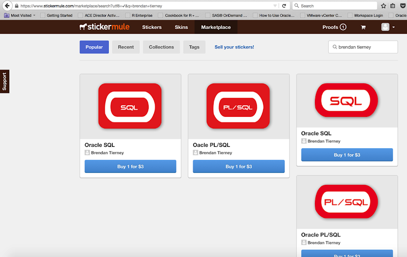
If you would like to get these as stickers and put them on your laptop, notebooks, or anywhere really, you can order them on Stickermule.

NewImage

NB: It is important to note that these are in no way approved or acknowledged or endorsed or anything else by Oracle.

Friday, October 9, 2015

From Zero to Dashboards in 10min with BICS

Unless you have been going around with your head in the clouds, all you can hear from all the big names in the IT worlds is about moving to the Cloud. (yes that was a poor attempt at a joke. It is Friday afternoon after all).

The title of this post is 'From Zero to Dashboards in 5 min with BICS'.

BICS stands for Oracle BI Cloud Service.

Over the past few months I've been working rolling out BICS at a number of different sites, and it is surprising how quickly you can get up and running with BICS.

There is no install. There is the minimum of setup and configuration. All you need to do is to create a user and give them some privileges. All of that takes 2 minutes.

Next get them to log in to BICS (2 minutes for the first time they log in) and load up some data using the Data Load feature (another 2 minutes).

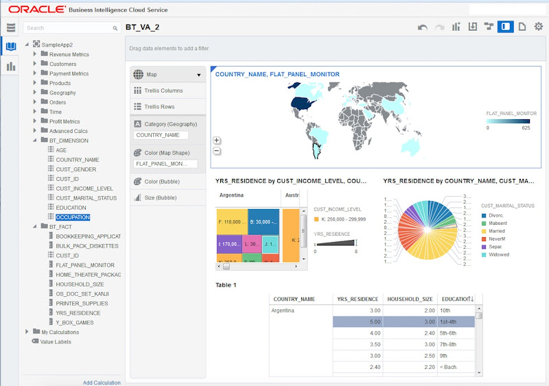
Then you can move onto the fun part of creating some Dashboards using Visual Analyzer. See the example below of one that we created in 4 minutes.

Bics 1

So all of the above took 10 minutes. How quick and easy is that!

Give it a go yourself and see how quick it is for you.

Let me know if you have any question on using BICS and if you need any help.

Tuesday, September 8, 2015

24th Sept: Oracle UG Ireland: BA, Big Data & Tech SIG (Free) event

This is a Free Event.

Register today to reserve your place, as places are limited.

Our next BA, Big Data & Tech SIG will be on Thursday 24th September. This event will be held in Jurys Inn, Customs House, in Dublin.

We have decided to merge the two SIGs for this event to offer everyone even more content and learning opportunities. The day is filled with presentations from End Users and from Product Experts. We will also have some of the latest updates from Oracle.

It is the ideal opportunity for you to learn, share and network with other users.

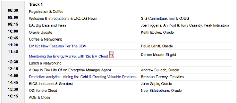
Here is the agenda for this full day event.

NewImage

As you can see this a really good agenda. So I hope to see you there.

You need to book your place for this SIG. To book your place go to here.


If you have ideas of topics you would like covered at the next SIG, just let me know.

I'll see you there.

Tuesday, September 1, 2015

My presentations at OOW 2015

Oracle Open World is coming at the end of October. Lots of people are starting to get excited as Oracle Open World is the number one place for all the Oracle geeks from around the World to hang out for a week.

This year I will be giving 2 presentations. Both of them are on the Sunday. That means I get to really enjoy the rest of the conference. These presentations are:

Sunday 13:30-14:15 & 14:30-15:14  (a double session)
Session Title : 12 more things about Oracle 12c 
Description: These sessions are being organised by the EMEA Oracle User Group and follow on from the successful sessions that were at last years Oracle Open World. These sessions/presentations will consist of 12 presenters giving a 5-7 minute talk on a topic related to the Oracle Database. Many thanks to Debra Lilley for arranging these session.  

For me I will be talking about Running R in the Oracle Database using Oracle R Enterprise. 5-7 Minutes is not enough time for this topic, but the whole idea of these sessions and talks to to give people a taster of what is possible in the Oracle Database. You can then use your new knowledge to check out other sessions at OOW and/or to check it out when you get home.

I'll put up another blog post when I have the full list and schedule of presenters.

Sunday 15:30-16:15  (yes this is right after the previous session/presentation)
Session Title : Real Business Value from Big Data and Advanced Analytics
Description : I will be co-presenting with Antony Heljula and we will be talking about some of the advanced analytics and big data projects we have worked on. We have had some amazing results with these projects and we will be giving you a taster of what is possible. Also some of these project didn't involve big data. So even with small data you can have amazing results using Advanced Analytics / Predictive Analytics / Data Mining / Data Science.

After these presentations I get to enjoy the rest of Oracle Open World with having to worry about giving another presentation.

My diary for the conference is filling up fast and it looks like I will be busy each day from 8am to late into the evening. Oracle Open World has lots and lots of social and networking events and these are great for meeting up with people and making new contacts.

Wednesday, August 26, 2015

Enabling Autotrace in SQL Developer

This is mainly a note to myself to save me from looking up the details very time I need it. I can just go to my own post.

To use Autotrace in SQL you need to grant the schema the PLUSTRACE role.

But in SQL Developer you need the PLUSTRACE role that has a few additional privileges.

Connect to SYS as sysdba and run the following.

grant select on v_$session to plustrace;
grant select on v_$sql_plan to plustrace;
grant select on v_$sql_plan_statistics to plustrace;
grant select on v_$sql to plustrace;

Now you will be able to run Autotrace in SQL Developer.

(Make sure to reconnect your SQL Developer connection so that the privileges can be picked up).

Friday, August 14, 2015

Managing ORE in-database Data Stores using SQL

When working with ORE you will end up creating a number of different data stores in the database. Also as your data science team increases the number of data stores can grow to a very large number.

When you install Oracle R Enterprise you will get a number of views that are made available to ORE users to see what ORE Data stores they have and what objects exist in them. All using SQL.

Perhaps some of the time the ORE developers and data analysts will use the set of ORE functions to manage the in-database ORE Data stores. These include:

NewImage

When using these ORE function the schema user/data scientist can see what ORE Data stores they have. You can use the ore.delete to delete an ORE Data store when it is no longer needed.

But the problem here is that over time your schemas can get a bit clogged up with ORE Data stores. Particularly when the data scientist is not longer working on the project or there is no need to maintain ORE Data stores. This is common on data science projects when you might have a number of data scientists work in/sharing the one database schema.

For a DBA, who's role will be to clean up the ORE Data store that are no longer needed, you have 4 options.

The first of these, is if all the ORE Data stores exist in the data scientists schema and nothing else in the schema is needed then you can just go ahead and drop the schema.

The second option is to log into the schema using SQL and drop the ORE Data stores. See an example of this below.

The third option is to connect to the Oracle schema using R and ORE and then use the ore.delete function to drop the ORE Data stores.

The fourth option is to connect to the RQSYS schema. This schema is the owner of the views used to query the ORE Data stores in each schema. After the RQSYS schema was created it was locked as part of the ORE installation. You as the DBA will need to unlock and then connect.

The following SQL lists the ORE Data stores that were created for that schema.

column dsname format a20
column description format a35

SELECT * FROM rquser_DataStoreList;

DSNAME                     NOBJ     DSSIZE CDATE     DESCRIPTION
-------------------- ---------- ---------- --------- -----------------------------------
ORE_DS                        2       5104 04-AUG-15 Example of ORE Datastore
ORE_FOR_DELETION              1       1675 14-AUG-15 Need to Delete this ORE Datastore
ORE_DS2                       5   51466509 04-AUG-15 DS for all R Env Data

You can also view what objects have saved in the ORE Data store.

column objname format a15
column class format a15
SELECT * FROM rquser_DataStoreContents;
 
DSNAME               OBJNAME         CLASS              OBJSIZE     LENGTH       NROW       NCOL
-------------------- --------------- --------------- ---------- ---------- ---------- ----------
ORE_DS               CARS_DATA       ore.frame             1306         11         32         11
ORE_DS               cars_ds         data.frame            3798         11         32         11
ORE_DS2              cars_ds         data.frame            3798         11         32         11
ORE_DS2              cars_ore_ds     ore.frame             1675         11         32         11
ORE_DS2              sales_ds        data.frame        51455575          7     918843          7
ORE_DS2              usa_ds          ore.frame             2749         23      18520         23
ORE_DS2              usa_ds2         ore.frame             2712         23      18520         23
ORE_FOR_DELETION     cars_ore_ds     ore.frame             1675         11         32         11

To drop an ORE Data store for you current schema you can use the rqDropDataStore SQL function.

BEGIN
   rqDropDataStore('ORE_FOR_DELETION');
END;
/

For the DBA when you unlock and connect to the RQSYS schema you will be able to see all the ORE Data stores in the data. The views will contain an additional column.

But if you use the above SQL function to delete an ORE Data store it will not work. This because this SQL function will only drop and ORE Data store if it exists in your schema. If we have connected to the RQSYS schema we will not have any ORE Data stores in it.

We can create a procedure that will allow use to delete/drop any ORE Data store in any schema.

create or replace PROCEDURE my_ORE_Datastore_Drop(
  ds_owner  in VARCHAR2,
  ds_name  IN VARCHAR2
  )
IS
  del_objIds rqNumericSet;
BEGIN
  del_objIds := rq$DropDataStoreImpl(ds_owner, ds_name);
  IF del_objIds IS NULL THEN
    raise_application_error(-20101, 'DataStore ' ||
                            ds_name || ' does not exist');
  END IF;

  -- remove from rq$datastoreinventory
  BEGIN
    execute immediate
       'delete from RQ$DATASTOREINVENTORY c where c.objID IN (' ||
       'select column_value from table(:del_objIds))' using del_objIds;
     COMMIT;
  EXCEPTION WHEN others THEN null;
  END;
END;

We are the DBA, logged into the RQSYS schema can now delete any ORE Data store in the database, using the following.

BEGIN
   my_ORE_Datastore_Drop('ORE_USER', 'ORE_FOR_DELETION');
END;
/

Thursday, July 30, 2015

Check out What Sauron is saying about Oracle

Over past year we have been (hopefully) hearing about Oracle Big Data SQL.

This is a new(-ish) option from Oracle that allows us to run our SQL queries not just on the data in our Oracle Database but also against NoSQL databases and Hadoop. No extra coding is needed, no extra formatting is needed, etc.

All the hard work in connecting to the data in this systems, translating it into executable code on these systems, executing it, capturing the results and presenting the results back to us sitting in our schema in our Oracle Database.

How cool is that.

To learn more about Oracle Big Data SQL check out their webpage.

But what let us get back to the title of this blog post, 'What Sauron is saying about Oracle'. I used these back at one of my presentation at BIWA Summit in January 2015 and I've been meaning to post these since.

If you have read books or watch the movies you will remember the phrase.

NewImage

We can apply this phrase to Oracle SQL now.

NewImage

or maybe my alternative version might be better.

NewImage

Tuesday, July 28, 2015

Charting Number of R Packages over time (Part 3)

This is the third and final blog post on analysing the number of new R packages that have been submitted over time.

Check out the previous blog posts:

In this blog post I will show you how you can perform Forecasting on our data to make some predictions on the possible number of new packages over the next 12 months.

There are 2 important points to note here:

  1. Only time will tell if these predictions are correct or nearly connect. Just like with any other prediction techniques.
  2. You cannot use just one of the Forecasting techniques in isolation to make a prediction. You need to use a number of functions/algorithms to see which one suits your data best.

The second point above is very important with all prediction techniques. Sometimes you see people/articles talking about them only using algorithm X. They have not considered any of the other techniques/algorithms. It is their favourite or preferred method. But that does not mean it works or is suitable for all data sets and all scenarios.

In this blog post I'm going to use 3 different forecasting functions, the in-build Forecast function in R, using HoltWinters and finally using ARIMA. Yes there are many more (it is R after all) and I'll leave these for you to explore.

1. Convert data set to Time Series data format

The first thing I need to do is to convert the data I want analyze into TimeSeries format (ts). This looks to have one record or instance for each data point.

So you cannot not have any missing data, or in my case any missing dates. Yes (for my data set) we could have some months where we do not have any submissions. What I could do is to work out mean values (or things like that) and fill for the missing months. But I'm feeling a bit lazy and after examining the data I see that we have a continuous set of data from September 2009 onwards. This is fine as most of the growth up to that point is flat.

So I need to subset the data to only include cases greater than or equal to September 2009 and less than or equal to June 2015. I wanted to explore July 2015 as the number for this month is incomplete.

The following code builds on the work we did in the second blog post in the series

library(forecast)
library(ggplot2)

# Subset the data
sub_data <- subset(data.sum, Group.date >= as.Date("2009-08-01", "%Y-%m-%d"))
sub_data <- subset(sub_data, Group.date <= as.Date("2015-06-01", "%Y-%m-%d"))

# Subset again to only take out the data we want to use in the time series
sub_data2 <- sub_data[,c("R_NUM")]

# Create the time series data, stating that it is monthly (12) and giving the start and end dates
ts_data <- ts(sub_data2, frequency=12, start=c(2009, 8), end=c(2015, 6))

# View the time series data
ts_data
     Jan Feb Mar Apr May Jun Jul Aug Sep Oct Nov Dec
2009                               2   3   4   3   4
2010   5   5   1  11   5   2   5   4   4   5   1   3
2011  11   4   3   6   6   5   9  15   5   8  23  18
2012  33  17  51  28  37  33  50  71  41 231  51  60
2013  75  67  76  81  76  74  77  89 111  96 111 200
2014 155 129 175 140 145 133 155 207 232 162 229 310
2015 308 343 332 378 418 558    

We now have the data prepared for input to our Forecasting functions in R.

2. Using Forecast in R

For the Forecast function all you need to do is pass in the Time Series dataset and tell the function how my steps into the future you want it to predict. In all my examples I'll ask the functions to predict for the next 12 months.

ts_forecast <- forecast(ts_data, h=12)
ts_forecast

         Point Forecast     Lo 80     Hi 80 Lo 95     Hi 95
Jul 2015       447.1965  95.67066  784.3163     0  958.6669
Aug 2015       499.4344 115.94329  873.1822     0 1069.8689
Sep 2015       551.7875 123.88426  952.0773     0 1230.4707
Oct 2015       603.7212 156.89486 1078.0395     0 1370.2069
Nov 2015       654.7647 143.29718 1179.4903     0 1603.8335
Dec 2015       704.5162 135.76829 1352.8925     0 1844.7230
Jan 2016       752.6447 151.09936 1502.6088     0 2100.9708
Feb 2016       798.8877 156.37383 1652.0847     0 2575.3715
Mar 2016       843.0474 159.67095 1848.1703     0 2888.1738
Apr 2016       884.9849 154.59456 2061.7990     0 3281.6062
May 2016       924.6136 148.04651 2325.9060     0 3891.5064
Jun 2016       961.8922 138.67935 2531.7578     0 4395.6033

plot(ts_forecast)

NewImage

For this we get a very large range of values and very wide predictive intervals. If we limit the y axis we can get a better picture of the actual predictions.

plot(ts_forecast, ylim=range(0:1000))
NewImage

3. Using HoltWinters

For HoltWinters we can use the in-built R function for this. All we need to do is to pass in the Time Series data set. The first part we can plot the HoltWinters for the existing data set

?HoltWinters
hw <- HoltWinters(ts_data)
plot(hw)
NewImage

Now we want to predict for the next 12 months

forecast <- predict(hw, n.ahead = 12, prediction.interval = T, level = 0.95)
forecast

              fit       upr      lwr
Jul 2015 519.9304  599.8097 440.0512
Aug 2015 560.1083  648.4183 471.7983
Sep 2015 601.4528  701.0163 501.8892
Oct 2015 643.9639  757.3750 530.5529
Nov 2015 681.5168  811.0727 551.9608
Dec 2015 724.7363  872.4508 577.0218
Jan 2016 773.8308  941.4768 606.1848
Feb 2016 809.8836  999.0401 620.7272
Mar 2016 847.1448 1059.2371 635.0525
Apr 2016 898.4476 1134.7795 662.1158
May 2016 933.8755 1195.6532 672.0977
Jun 2016 972.3866 1260.7376 684.0356

plot(hw, forecast)
NewImage

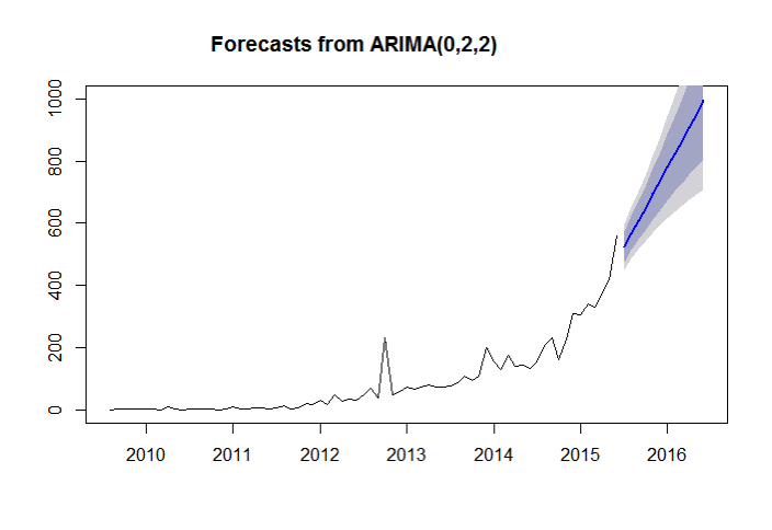
4. Using ARIMA

For ARIMA we need to perform a simple conversion of the Time Series data into ARIMA format and then perform the forecase

fc_arima <- auto.arima(ts_data)
fc_fc_arima  <- forecast(fc_arima, h=12)
fc_fc_arima

         Point Forecast    Lo 80     Hi 80    Lo 95     Hi 95
Jul 2015       524.4758 476.2203  572.7314 450.6753  598.2764
Aug 2015       567.1156 513.2301  621.0012 484.7048  649.5265
Sep 2015       609.7554 548.3239  671.1869 515.8041  703.7068
Oct 2015       652.3952 581.6843  723.1062 544.2522  760.5383
Nov 2015       695.0350 613.5293  776.5408 570.3828  819.6873
Dec 2015       737.6748 644.0577  831.2920 594.4998  880.8499
Jan 2016       780.3147 673.4319  887.1974 616.8516  943.7777
Feb 2016       822.9545 701.7797  944.1292 637.6337 1008.2752
Mar 2016       865.5943 729.2004 1001.9881 656.9978 1074.1907
Apr 2016       908.2341 755.7718 1060.6963 675.0631 1141.4050
May 2016       950.8739 781.5559 1120.1918 691.9244 1209.8233
Jun 2016       993.5137 806.6027 1180.4246 707.6581 1279.3693

plot(fc_fc_arima, ylim=range(0:800))
NewImage

As you can see there are very different results from each of these forecasting techniques. If this was a real life project on real data then we would go about exploring a lot more of the Forecasting function available in R. The reason for this is to identify which R function and Forecasting algorithm works best for our data.

Which Forecasting technique would you choose from the selection above?

But will this function and algorithm always work with our data? The answer is NO. As our data evolves so may the algorithm that works best for our data. This is why the data science/analytics world is iterative. We need to recheck/revalidate the functions/algorithms to see if we need to start using something else or not. When we do need to use another function/algorithm you need to ask yourself why this has happened, what has changed in the data, what has changed in the business, etc.

Wednesday, July 22, 2015

Charting Number of R Packages over time (Part 2)

This is the second blog post on charting the number of new R Packages over time.

Check out the first blog post that looked at getting the data, performing some simple graphing and then researching some issues that were identified using the graph.

In this blog post I will look at how you can aggregate the data, plot it, get a regression line, then plot it using ggplot2 and we will include a trend line using the geom_smooth.

1. Prepare the data

In my previous post we extracted and aggregated the data on a daily bases. This is the plot that was shown in my previous post. This gives us a very low level graph and perhaps we might get something a little bit more useable is we aggregated the data. I have the data in an Oracle Database so it would be easy for me to write another query to perform the necessary aggregation. But let's make things a little bit trickier. I'm going to use R to do the aggregation.

Our data set is in the data frame called data. What I want to do is to aggregate it up to monthly level. The first thing I did was to create a new column that contains the values of the new aggregate level.

data$R_MONTH <- format(rdate2, "%Y%m01")
data$R_MONTH <- as.Date(data$R_MONTH3, "%Y%m%d")
data.sum <- aggregate(x = data[c("R_NUM")],
                    FUN = sum,
                    by = list(Group.date = data$R_MONTH)
)

2. Plot the Data

We now have the data aggregated at monthly level. We can now plot the graph. Ignore the last data point on the chart. This is for July 2015 and I extracted the data on the 9th of July. So we do not have a full months of data here.

plot(as.Date(data.sum$Group.date), data.sum$R_NUM, type="b", xaxt="n", cex=0.75 , ylab="Num New Packages", main="Number of New Packages by Month")
axis(1, as.Date(data.sum$Group.date, "%Y-%d"), as.Date(data.sum$Group.date, "%Y-%d"), cex.axis=0.5, las=1)

This gives us the following graph.

NewImage

3. Plot the data using ggplot2

The basic plot function of R is great and allows us to quickly and easily get some good graphs produced. But it is a bit limited and perhaps we want to create something that is a bit more elaborate. ggplot2 is a very popular package that can allow us to create a graph, building it up in a number of steps and layers to give something that is a lot more professional.

In the following example I've kept things simple and Yes I could have done so much more. I'll leave that as an exercise for you go off an do.

The first step is to use the qplot function to produce a basic plot using ggplot2. This gives us something similar to what we got from the plot function.

library(ggplot2)
qplot(x=factor(data.sum$Group.date), y=data.sum$R_NUM, data=data.sum, 
       xlab="Year/Month", ylab='Num of New Packages', asp=0.5)

This gives us the following graph.

NewImage

Now if we use ggplot2 then we need to specify a lot more information. Here is the equivalent plot using ggplot2 (with a line plot).

NewImage

4. Include a trend line

We can very easily include a trend line in a ggplot2 graph using the geom_smooth command. In the following example we have the same chart and include a linear regression line.

plt <- ggplot(data.sum, aes(x=factor(data.sum$Group.date), y=data.sum$R_NUM)) + geom_line(aes(group=1)) +
  theme(text = element_text(size=7),
        axis.text.x = element_text(angle=90, vjust=1)) + xlab("Year / Month") + ylab("Num of New Packages") +
  geom_smooth(method='lm', se=TRUE, size = 0.75, fullrange=TRUE, aes(group=20))
plt

NewImage

We can tell a lot from this regression plot.

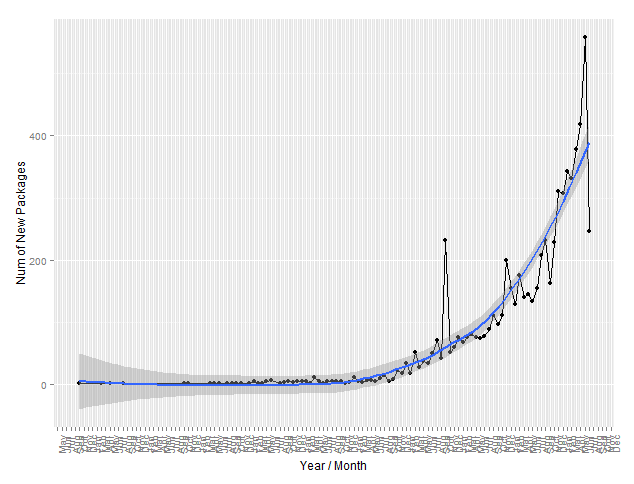
But perhaps we would like to see a trend line on the chart, with something like a moving averages plot. Plus I've added in a bit of scaling to help with representing the data at a monthly level.

library(scales)
plt <- ggplot(data.sum, aes(x=as.POSIXct(data.sum$Group.date), y=data.sum$R_NUM)) + geom_line() + geom_point() +
  theme(text = element_text(size=12),
        axis.text.x = element_text(angle=90, vjust=1)) + xlab("Year / Month") + ylab("Num of New Packages") +
  geom_smooth(method='loess', se=TRUE, size = 0.75, fullrange=TRUE) +
  scale_x_datetime(breaks = date_breaks("months"), labels = date_format("%b"))
plt
NewImage

In the third blog post on this topic I will look at how we can use some of the forecasting and predicting functions available in R. We can use these to see help us visualize what the future growth patterns might be for this data. I have some interesting things to show.