This Blog has moved platform - Check it out

 I've moved this blog to Wordpress platform.  Go check it out as it will have lots and lots of newer materials and blog posts, as well as all the blog posts from this site.  So the newer site is bigger and better.

Go to -  www.oralytics.com

Machine Learning Tools and Workbenches

The following is a list of the most commonly used tools and workbenches for machine learning. These are specific to machine learning only. This list does not include any library or frameworks. These are tools and workbenches only. Most offering machine learning tools will include the following features:

• Easy drag and drop capabilities
• Data collection
• Data preparation and cleaning
• Model building
• Data Visualization
• Model Deployment
• Integration with other tools and languages

As more and more organizations implement machine learning, there are two core aims they want to achieve.

1. Employee Productivity: Who wants to spend days or weeks writing mundane code to load data, clean data, etc etc etc. No one wants to do this and especially employers don’t want their staff wasting time on this. Instead they are happy to invest in tools and workbenches where a lot or most or all of these mundane tasks are automated for you. You can not concentrate on the important tasks of adding value to your organisation. This saves money, improves employee productivity and employee value.
2. Integration with Technical Architecture: Many of these tools and workbenches allow for easy integration with the technical architecture and thereby allowing easy and quick integration of machine learning withe the day to day activities of the organization. This saves money, improves employee productivity and employee value.

SAS
SAS software has been around for every and is the great grand-daddy of analytics and machine learning. They have built a large number of machine learning tools and solutions built upon these for various industries. Their core machine learning tools include SAS Enterprise Miner and SAS Visual Data Mining and Machine Learning.

Microsoft
Microsoft have been improving their Machine Learning offering over the years and most of this is based on the Azure cloud platform with Microsoft Azure Machine Learning Studio and Azure Databricks.

SAP
SAP Leonardo is a cloud based platform for machine learning and supports tight integration with other SAP software.

Oracle
Oracle have a number of machine learning tools and supports for the main machine learning languages. They have built a large number of applications (both cloud and on-premises) with in-built machine learning. Their main tools for machine learning include Oracle Data Miner, Oracle Machine Learning and Oracle Analytics (OAC or DVD versions)

Cloudera
If you work with hadoop and big data then you are probably using Cloudera in some way. Cloudera have hired Hilary Mason as their GM of ML. By taking an “AI factory” approach to turning data into decisions, you can make the process of building, scaling, and deploying enterprise ML and AI solutions automated, repeatable, and predictable—boring even. Cloudera Data Science Workbench is their solution.


IBM
IBM have a number of machine learning tools, one of them being a long standing member of the machine learning community, SPSS Modeler. Other machine learning tools include Watson Studio, IBM Machine Learning for z/OS, and IBM Watson Explorer.

Google
Google have a large number of machine learning solutions including everything from traditional machine learning, into NLP, in Image processing, Video processing, etc. It’s a long list. Many of these come with various APIs to access these features. Most of these revolve around their Google AI Cloud offering. But sticking with the tools and workbenches we have AI Platform Notebooks, Kubeflow, and BigQuery ML.

TensorBoard
TensorBoard is a suite of tools for graphical representation of different aspects and stages of machine learning in TensorFlow.

Amazon
A bit like Goolge, Amazon has a large number of solutions for machine learning and AI, and most of these are available via an API or some cloud service. Amazon SageMaker is their main service.

Looker
Looker connects directly with Google BQML reduces additional complexity for data scientists by eliminating the need to move outputs of predictive models back into the database for use, while also increases the time-to-value for business users, allowing them to operationalize the outputs of predictive metrics to make better decisions every day.

Weka
Weka has been around for a long time and still popular in some research groups. Weka is a collection of machine learning algorithms for data mining tasks. It contains tools for data preparation, classification, regression, clustering, association rules mining, and visualization.

 






RapidMiner
RapidMiner Studio has been around for a long time and is one of the few more visual workflow tools (that everyone else should be doing).

Databricks
From the people who created Spark, we have another notebook solution for your machine learning projects called Databricks Workbench.

KNIME
KNIME Analytics Platform is the open source software for creating data science applications and services.

Dataiku
Dataiki Data Science (DSS) is a collaborative data science software workflow platform enabling data exploration, prototyping and delivery of analytical and machine learning solutions.

I’ve not included the tools like R Studio and Notebooks in this list as they don’t really address the aims listed above. But you will notice a lot of the above solutions are really Jupyter Notebooks. Most of these vendors have a long way to go to make the tasks of machine learning boring.

This list does not cover all available tools and workbenches, but it does list the most common one you will come across.

Time Series Forecasting in Oracle – Part 2

This is the second part about time-series data modeling using Oracle. Check out the first part here.

In this post I will take a time-series data set and using the in-database time-series functions model the data, that in turn can be used for predicting future values and trends.

The data set used in these examples is the Rossmann Store Sales data set. It is available on Kaggle and was used in one of their competitions.

Let's start by aggregating the data to monthly level. We get.
 

Data Set-up
Although not strictly necessary, but it can be useful to create a subset of your time-series data to only contain the time related attribute and the attribute containing the data to model. When working with time-series data, the exponential smoothing function expects the time attribute to be of DATE data type. In most cases it does. When it is a DATE, the function will know how to process this and all you need to do is to tell the function the interval. A view is created to contain the monthly aggregated data.

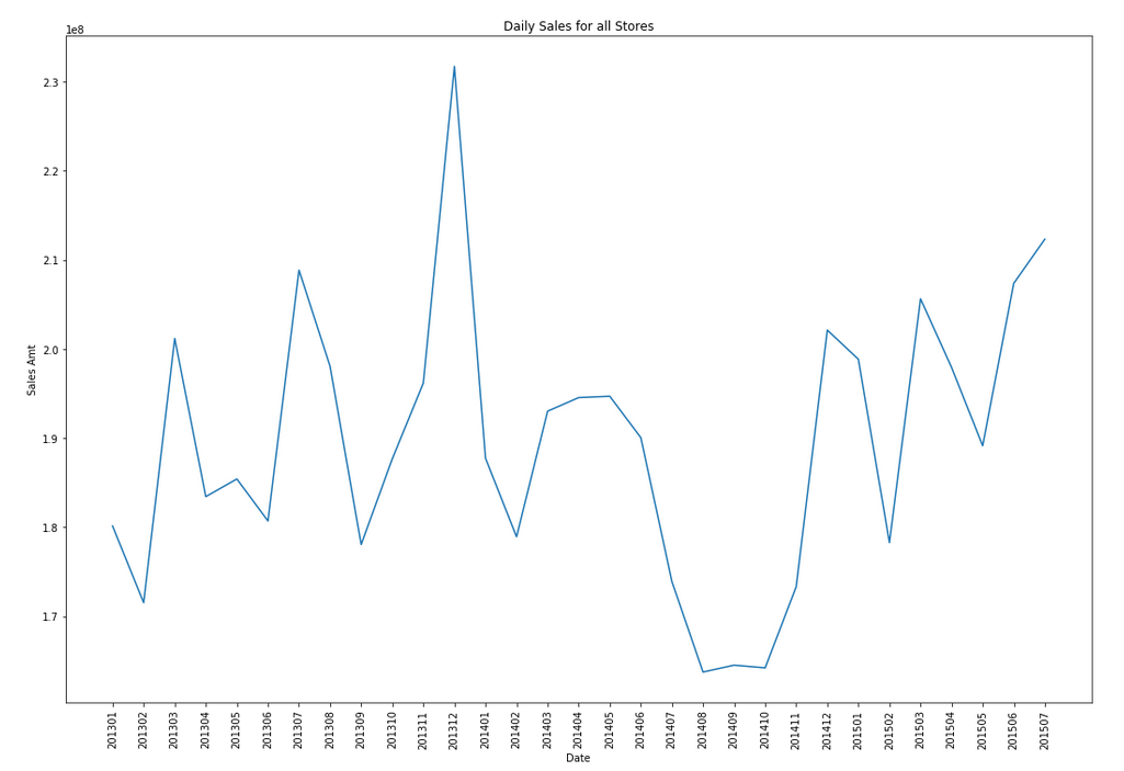
-- Create input time series
create or replace view demo_ts_data as 
select to_date(to_char(sales_date, 'MON-RRRR'),'MON-RRRR') sales_date,
sum(sales_amt) sales_amt
from demo_time_series
group by to_char(sales_date, 'MON-RRRR')
order by 1 asc;

Next a table is needed to contain the various settings for the exponential smoothing function.

CREATE TABLE demo_ts_settings(setting_name VARCHAR2(30), 
                              setting_value VARCHAR2(128));

Some care is needed with selecting the parameters and their settings as not all combinations can be used.

Example 1 - Holt-Winters
The first example is to create a Holt-Winters time-series model for hour data set. For this we need to set the parameter to include defining the algorithm name, the specific time-series model to use (exsm_holt), the type/size of interval (monthly) and the number of predictions to make into the future, pass the last data point.

BEGIN
   -- delete previous setttings
   delete from demo_ts_settings;

   -- set ESM as the algorithm
   insert into demo_ts_settings 
      values (dbms_data_mining.algo_name,
              dbms_data_mining.algo_exponential_smoothing);

   -- set ESM model to be Holt-Winters
   insert into demo_ts_settings 
      values (dbms_data_mining.exsm_model,
              dbms_data_mining.exsm_holt);

   -- set interval to be month
   insert into demo_ts_settings 
      values (dbms_data_mining.exsm_interval,
              dbms_data_mining.exsm_interval_month);

   -- set prediction to 4 steps ahead
   insert into demo_ts_settings 
      values (dbms_data_mining.exsm_prediction_step,
              '4');

   commit; 
END;

Now we can call the function, generate the model and produce the predicted values.

BEGIN
   -- delete the previous model with the same name
   BEGIN 
      dbms_data_mining.drop_model('DEMO_TS_MODEL');
   EXCEPTION 
      WHEN others THEN null; 
   END;

   dbms_data_mining.create_model(model_name => 'DEMO_TS_MODEL',
                                 mining_function => 'TIME_SERIES',
                                 data_table_name => 'DEMO_TS_DATA',
                                 case_id_column_name => 'SALES_DATE',
                                 target_column_name => 'SALES_AMT',
                                 settings_table_name => 'DEMO_TS_SETTINGS');
END;

When the model is create a number of data dictionary views are populated with model details and some addition views are created specific to the model. One such view commences with DM$VP. Views commencing with this contain the predicted values for our time-series model. You need to append the name of the model create, in our example DEMO_TS_MODEL.
 

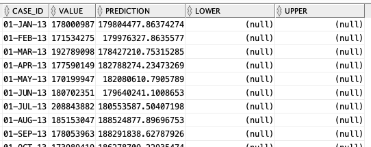
-- get predictions
select case_id, value, prediction, lower, upper 
from   DM$VPDEMO_TS_MODEL
order by case_id;

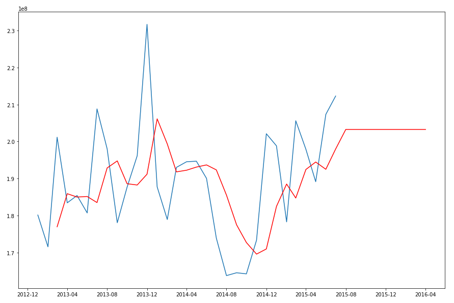
When we plot this data we get. The blue line contains the original data values and the red line contains the predicted values. The predictions are very similar to those produced using Holt-Winters in Python.  

Example 2 - Holt-Winters including Seasonality
The previous example didn't really include seasonality int the model and predictions. In this example we introduce seasonality to allow the model to pick up any trends in the data based on a defined period. For this example we will change the model name to HW_ADDSEA, and the season size to 5 units. A data set with a longer time period would illustrate the different seasons better but this gives you an idea.

BEGIN
   -- delete previous setttings
   delete from demo_ts_settings;

   -- select ESM as the algorithm
   insert into demo_ts_settings 
   values (dbms_data_mining.algo_name,
           dbms_data_mining.algo_exponential_smoothing);

   -- set ESM model to be Holt-Winters Seasonal Adjusted
   insert into demo_ts_settings 
   values (dbms_data_mining.exsm_model,
           dbms_data_mining.exsm_HW_ADDSEA);

   -- set interval to be month
   insert into demo_ts_settings 
   values (dbms_data_mining.exsm_interval,
   dbms_data_mining.exsm_interval_month);

  -- set prediction to 4 steps ahead
  insert into demo_ts_settings 
  values (dbms_data_mining.exsm_prediction_step,
          '4');

   -- set seasonal cycle to be 5 quarters
   insert into demo_ts_settings 
   values (dbms_data_mining.exsm_seasonality,
           '5');

commit; 
END;

We need to re-run the creation of the model and produce the predicted values. This code is unchanged from the previous example.

BEGIN
   -- delete the previous model with the same name
   BEGIN 
      dbms_data_mining.drop_model('DEMO_TS_MODEL');
   EXCEPTION 
      WHEN others THEN null; 
   END;

   dbms_data_mining.create_model(model_name => 'DEMO_TS_MODEL',
                                 mining_function => 'TIME_SERIES',
                                 data_table_name => 'DEMO_TS_DATA',
                                 case_id_column_name => 'SALES_DATE',
                                 target_column_name => 'SALES_AMT',
                                 settings_table_name => 'DEMO_TS_SETTINGS');
END;

When we re-query the DM$VPDEMO_TS_MODEL we get the new values. When plotted we get.
The blue line contains the original data values and the red line contains the predicted values.

Comparing this chart to the chart from the first example we can see there are some important differences between them. These differences are particularly evident in the second half of the chart, on the right hand side. We get to see there is a clearer dip in the predicted data. This mirrors the real data values better. We also see better predictions as the time line moves to the end.

When performing time-series analysis you really need to spend some time exploring the data, to understand what is happening, visualizing the data, seeing if you can identifying any patterns, before moving onto using the different models. Similarly you will need to explore the various time-series models available and the parameters, to see what works for your data and follow the patterns in your data. There is not magic solution in this case.

Data Sets for Analytics

When working with analytics, in whatever flavor, one of the key things you need is some data. But data comes in many different shapes and sizes, but where can you get some useful data, be it transactional, time-series, meta-data, analytical, master, categorical, numeric, regression, clustering, etc.

Many of the popular analytics languages have some data sets built into them. For example the R language comes pre-loaded with data sets and these can be accessed using

data()

but many of the R packages also come with data sets.

Similarly if you are using Python, it comes with some pre-loaded data sets and similarly many of the Python libraries have data sets build into them. For example scikit learn.

from sklearn import datasets

But where else can you get data sets. There are lots and lots of website available with data sets and the list could be very long. The following is a list of, what I consider, the websites with the best data sets.

Kaggle
Amazon Open Data
UCI Machine Learning Repository
Google Search Engine
Google Open Images Data
Google Fiance
Microsoft Open Data
Awesome Public Datasets Collection
EU Open Data
US Government Data
US Census Bureau
Ireland Open Data
Northern Ireland Public Open Data
UK Open Data
Image Processing Data
Carnegie Mellon University Data Sets
World Bank Open Data
IMF Open Data
Movie Reviews Data Set
Amazon Reviews
Amazon public data sets
IMDb Datasets

Time Series Forecasting in Oracle – Part 1

Time-series analysis comprises methods for analyzing time series data in order to extract meaningful statistics and other characteristics of the data. In this blog post I'll introduce what time-series analysis is, the different types of time-series analysis and introduce how you can do this using SQL and PL/SQL in Oracle Database. I'll have additional blog posts giving more detailed examples of Oracle functions and how they can be used for different time-series data problems. Time-series forecasting is the use of a model to predict future values based on previously observed/historical values. It is a form of regression analysis with additions to facilitate trends, seasonal effects and various other combinations.




Time-series forecasting is not an exact science but instead consists of a set of statistical tools and techniques that support human judgment and intuition, and only forms part of a solution. It can be used to automate the monitoring and control of data flows and can then indicate certain trends, alerts, rescheduling, etc., as in most business scenarios it is used for predict some future customer demand and/or products or services needs. Typical application areas of Time-series forecasting include:

• Operations management: forecast of product sales; demand for services
• Marketing: forecast of sales response to advertisement procedures, new promotions etc.
• Finance & Risk management: forecast returns from investments
• Economics: forecast of major economic variables, e.g. GDP, population growth, unemployment rates, inflation; useful for monetary & fiscal policy; budgeting plans & decisions
• Industrial Process Control: forecasts of the quality characteristics of a production process
• Demography: forecast of population; of demographic events (deaths, births, migration); useful for policy planning

When working with time-series data we are looking for a pattern or trend in the data. What we want to achieve is the find a way to model this pattern/trend and to then project this onto our data and into the future. The graphs in the following image illustrate examples of the different kinds of scenarios we want to model. [gallery ids="1360,1361,1362" type="rectangular"] Most time-series data sets will have one or more of the following components:

• Seasonal: Regularly occurring, systematic variation in a time series according to the time of year.
• Trend: The tendency of a variable to grow over time, either positively or negatively.
• Cycle: Cyclical patterns in a time series which are generally irregular in depth and duration. Such cycles often correspond to periods of economic expansion or contraction. Also know as the business cycle.
• Irregular: The Unexplained variation in a time series.

When approaching time-series problems you will use a combination of visualizations and time-series forecasting methods to examine the data and to build a suitable model. This is where the skills and experience of the data scientist becomes very important. Oracle provided a algorithm to support time-series analysis in Oracle 18c. This function is called Exponential Smoothing. This algorithm allows for a number of different types of time-series data and patterns, and provides a wide range of statistical measures to support the analysis and predictions, in a similar way to Holt-Winters.
 
The first parameter for the Exponential Smoothing function is the name of the model to use. Oracle provides a comprehensive list of models and these are listed in the following table.
 
Check out my other blog posts on performing time-series analysis using the Exponential Smoothing function in Oracle Database. These will give more detailed examples of how the Oracle time-series functions, using the Exponential Smoothing algorithm, can be used for different time-series data problems. I'll also look at example of the different configurations

Python transforming Categorical to Numeric

When preparing data for input to machine learning algorithms you may have to perform certain types of data preparation. In most enterprise solutions all or most of these tasks are automated for you, but in many languages they aren't. The enterprise solutions are about 'automating the boring stuff' so that you don't have to worry about it and waste valuable time doing boring, repetitive things. The following examples illustrates a number of ways to record categorical variables into numeric. There are a number of approaches available, and it is up to you to decide which one might work best for your problem, your data, etc. Let's begin by loading the data set to be used in these examples. It is a Video Games reviews data set.

# perform some Statistics on the items in a panda
import pandas as pd
import numpy as np
import matplotlib as plt
videoReview = pd.read_csv('/Users/brendan.tierney/Downloads/Video_Games_Sales_as_at_22_Dec_2016.csv') 
videoReview.head(10)

What are the data types of each variable

videoReview.dtypes

We don't want to work with all the data in these examples. We just want to concentrate on the categorical variables. Let's us create a subset of the dataframe to contains these.

df = videoReview.select_dtypes(include=['object']).copy()
df.head(10)

Now do a little data clean up by removing NaN (nulls)

df.dropna(inplace=True)
df.isnull().sum()

df.describe()

The above image shows the number of unique values in each of the variables. We will use Platform, Genre and Rating for the variable example below. Let us chart these variables.

#check the number of passengars for each variable 
import seaborn as sb
import matplotlib.pyplot as plt

plt.rcParams['figure.figsize'] = 10, 8

sb.countplot(x='Platform',data=df, palette='hls')

sb.countplot(x='Genre',data=df, palette='hls')

sb.countplot(x='Rating',data=df, palette='hls')

1-One-hot Coding

The first approach is to use the commonly used one-hot coding method. This will take a categorical variable and create a set of new variables corresponding with each distinct value in the variable, and then populate it with a binary value to indicate the original value.

#apply one-hot-coding to all the categorical variables
# and create a new dataframe to store the results

df2 = pd.get_dummies(df)
df2.head(10)

As you can see we now have 8138 variables in the pandas dataframe! That is a lot and may not be workable for you. You may need to look at some feature reduction methods to reduce the number of variables. 2-Find and Replace In this example we will simple replace the values with defined values. Let's have a look at values in the Ratings variable and their frequencies.

df['Rating'].value_counts()

The last 4 values listed have very small number of occurrences. We will group these into having one value/category.

find_replace = {"Rating" : {"E": 1, "T": 2, "M": 3, "E10+": 4, "EC": 5, "K-A": 5, "RP": 5, "AO": 5}}
df.replace(find_replace, inplace=True)
df.head(10)

Now plot the newly generated rating values and their frequencies.

sb.countplot(x='Rating',data=df, palette='hls')

3 - Label encoding

With this technique where each distinct value in a categorical variable is converted to a number. In this scenario you don't get to pick the numeric value assigned to the value. It is system determined.

#let's check the data types again
df.dtypes

Our categorical variables are of 'object' data type. We need to convert to a category data type. In this example 'Platform' as it has a large-ish number of values and we want a quick way of converting them we can illustrate this by creating a new variable.

df["Platform_Category"] = df["Platform"].astype('category')
df.dtypes

Now convert this new variable to numeric.

df["Platform_Category"] = df["Platform_Category"].cat.codes
df.head(20)

The number assigned to the Platform_Category variable is based on the alphabetical ordering of the values in the Platform variable. For example,

df.groupby("Platform")["Platform"].count()

 

4-Using SciKit-Learn transform

SciKit-Learn has a number of functions to help with data encodings. The first one we will look at is the 'fit_transform' function. This will perform a similar task to what we have seen in a previous example.

#Let's use the fit_tranforms function to encode the Genre variable
from sklearn.preprocessing import LabelEncoder

le_make = LabelEncoder()
df["Genre_Code"] = le_make.fit_transform(df["Genre"])
df[["Genre", "Genre_Code"]].head(10)

And we can see this comparison when we look at the frequency counts.

df.groupby("Genre_Code")["Genre_Code"].count()

df.head(10)

And now we can drop the Genre variable from the dataframe as it is no longer needed. BUT you will need to have recorded the mapping between the original Genre values and the numeric values for future reference.

df = df.drop('Genre', axis=1)
df.head(10)

 

5-Using SciKit-Learn LabelEndcoder

SciKit-Learn has a binary label encoder and it can be used in a similar way to the previous example and also similar to the 'get_dummies' function.

from sklearn.preprocessing import LabelBinarizer

lb_style = LabelBinarizer()
lb_results = lb_style.fit_transform(df["Rating"])
lb_df = pd.DataFrame(lb_results, columns=lb_style.classes_)
lb_df.head(10)

These can now be joined with the original dataframe or a with a subset of the original dataframe to form a new dataframe consisting of the required variables. As you can see, from the following, there are several other data pre-processing functions available in SciKit-Learn.