Monday, April 15, 2019

Time Series Forecasting in Oracle – Part 1

Time-series analysis comprises methods for analyzing time series data in order to extract meaningful statistics and other characteristics of the data. In this blog post I'll introduce what time-series analysis is, the different types of time-series analysis and introduce how you can do this using SQL and PL/SQL in Oracle Database. I'll have additional blog posts giving more detailed examples of Oracle functions and how they can be used for different time-series data problems. Time-series forecasting is the use of a model to predict future values based on previously observed/historical values. It is a form of regression analysis with additions to facilitate trends, seasonal effects and various other combinations.


Screenshot 2019-04-13 12.59.56

Time-series forecasting is not an exact science but instead consists of a set of statistical tools and techniques that support human judgment and intuition, and only forms part of a solution. It can be used to automate the monitoring and control of data flows and can then indicate certain trends, alerts, rescheduling, etc., as in most business scenarios it is used for predict some future customer demand and/or products or services needs. Typical application areas of Time-series forecasting include:
  • Operations management: forecast of product sales; demand for services
  • Marketing: forecast of sales response to advertisement procedures, new promotions etc.
  • Finance & Risk management: forecast returns from investments
  • Economics: forecast of major economic variables, e.g. GDP, population growth, unemployment rates, inflation; useful for monetary & fiscal policy; budgeting plans & decisions
  • Industrial Process Control: forecasts of the quality characteristics of a production process
  • Demography: forecast of population; of demographic events (deaths, births, migration); useful for policy planning
When working with time-series data we are looking for a pattern or trend in the data. What we want to achieve is the find a way to model this pattern/trend and to then project this onto our data and into the future. The graphs in the following image illustrate examples of the different kinds of scenarios we want to model. [gallery ids="1360,1361,1362" type="rectangular"] Most time-series data sets will have one or more of the following components:
  • Seasonal: Regularly occurring, systematic variation in a time series according to the time of year.
  • Trend: The tendency of a variable to grow over time, either positively or negatively.
  • Cycle: Cyclical patterns in a time series which are generally irregular in depth and duration. Such cycles often correspond to periods of economic expansion or contraction. Also know as the business cycle.
  • Irregular: The Unexplained variation in a time series.
When approaching time-series problems you will use a combination of visualizations and time-series forecasting methods to examine the data and to build a suitable model. This is where the skills and experience of the data scientist becomes very important. Oracle provided a algorithm to support time-series analysis in Oracle 18c. This function is called Exponential Smoothing. This algorithm allows for a number of different types of time-series data and patterns, and provides a wide range of statistical measures to support the analysis and predictions, in a similar way to Holt-Winters.
 Screenshot 2019-04-15 11.57.40
The first parameter for the Exponential Smoothing function is the name of the model to use. Oracle provides a comprehensive list of models and these are listed in the following table.
 Screenshot 2019-04-15 11.57.40
Check out my other blog posts on performing time-series analysis using the Exponential Smoothing function in Oracle Database. These will give more detailed examples of how the Oracle time-series functions, using the Exponential Smoothing algorithm, can be used for different time-series data problems. I'll also look at example of the different configurations

Monday, April 8, 2019

Python transforming Categorical to Numeric

When preparing data for input to machine learning algorithms you may have to perform certain types of data preparation. In most enterprise solutions all or most of these tasks are automated for you, but in many languages they aren't. The enterprise solutions are about 'automating the boring stuff' so that you don't have to worry about it and waste valuable time doing boring, repetitive things. The following examples illustrates a number of ways to record categorical variables into numeric. There are a number of approaches available, and it is up to you to decide which one might work best for your problem, your data, etc. Let's begin by loading the data set to be used in these examples. It is a Video Games reviews data set.

# perform some Statistics on the items in a panda
import pandas as pd
import numpy as np
import matplotlib as plt
videoReview = pd.read_csv('/Users/brendan.tierney/Downloads/Video_Games_Sales_as_at_22_Dec_2016.csv') 
videoReview.head(10)


What are the data types of each variable

videoReview.dtypes


We don't want to work with all the data in these examples. We just want to concentrate on the categorical variables. Let's us create a subset of the dataframe to contains these.

df = videoReview.select_dtypes(include=['object']).copy()
df.head(10)


Now do a little data clean up by removing NaN (nulls)

df.dropna(inplace=True)
df.isnull().sum()

df.describe()


The above image shows the number of unique values in each of the variables. We will use Platform, Genre and Rating for the variable example below. Let us chart these variables.

#check the number of passengars for each variable 
import seaborn as sb
import matplotlib.pyplot as plt

plt.rcParams['figure.figsize'] = 10, 8

sb.countplot(x='Platform',data=df, palette='hls')


sb.countplot(x='Genre',data=df, palette='hls')


sb.countplot(x='Rating',data=df, palette='hls')

1-One-hot Coding

The first approach is to use the commonly used one-hot coding method. This will take a categorical variable and create a set of new variables corresponding with each distinct value in the variable, and then populate it with a binary value to indicate the original value.

#apply one-hot-coding to all the categorical variables
# and create a new dataframe to store the results

df2 = pd.get_dummies(df)
df2.head(10)


As you can see we now have 8138 variables in the pandas dataframe! That is a lot and may not be workable for you. You may need to look at some feature reduction methods to reduce the number of variables. 2-Find and Replace In this example we will simple replace the values with defined values. Let's have a look at values in the Ratings variable and their frequencies.

df['Rating'].value_counts()


The last 4 values listed have very small number of occurrences. We will group these into having one value/category.

find_replace = {"Rating" : {"E": 1, "T": 2, "M": 3, "E10+": 4, "EC": 5, "K-A": 5, "RP": 5, "AO": 5}}
df.replace(find_replace, inplace=True)
df.head(10)


Now plot the newly generated rating values and their frequencies.

sb.countplot(x='Rating',data=df, palette='hls')

3 - Label encoding

With this technique where each distinct value in a categorical variable is converted to a number. In this scenario you don't get to pick the numeric value assigned to the value. It is system determined.

#let's check the data types again
df.dtypes


Our categorical variables are of 'object' data type. We need to convert to a category data type. In this example 'Platform' as it has a large-ish number of values and we want a quick way of converting them we can illustrate this by creating a new variable.

df["Platform_Category"] = df["Platform"].astype('category')
df.dtypes


Now convert this new variable to numeric.

df["Platform_Category"] = df["Platform_Category"].cat.codes
df.head(20)


The number assigned to the Platform_Category variable is based on the alphabetical ordering of the values in the Platform variable. For example,

df.groupby("Platform")["Platform"].count()
 

4-Using SciKit-Learn transform

SciKit-Learn has a number of functions to help with data encodings. The first one we will look at is the 'fit_transform' function. This will perform a similar task to what we have seen in a previous example.

#Let's use the fit_tranforms function to encode the Genre variable
from sklearn.preprocessing import LabelEncoder

le_make = LabelEncoder()
df["Genre_Code"] = le_make.fit_transform(df["Genre"])
df[["Genre", "Genre_Code"]].head(10)


And we can see this comparison when we look at the frequency counts.

df.groupby("Genre_Code")["Genre_Code"].count()

df.head(10)


And now we can drop the Genre variable from the dataframe as it is no longer needed. BUT you will need to have recorded the mapping between the original Genre values and the numeric values for future reference.

df = df.drop('Genre', axis=1)
df.head(10)
 

5-Using SciKit-Learn LabelEndcoder

SciKit-Learn has a binary label encoder and it can be used in a similar way to the previous example and also similar to the 'get_dummies' function.

from sklearn.preprocessing import LabelBinarizer

lb_style = LabelBinarizer()
lb_results = lb_style.fit_transform(df["Rating"])
lb_df = pd.DataFrame(lb_results, columns=lb_style.classes_)
lb_df.head(10)


These can now be joined with the original dataframe or a with a subset of the original dataframe to form a new dataframe consisting of the required variables. As you can see, from the following, there are several other data pre-processing functions available in SciKit-Learn.

Monday, April 1, 2019

Data Normalization in Oracle Data Mining

Normalization is the process of scaling continuous values down to a specific range, often between zero and one. Normalization transforms each numerical value by subtracting a number, called the shift, and dividing the result by another number called the scale. The normalization techniques include:
  • Min-Max Normalization : There is where the normalization is based on the using the minimum value for the shift and the (maximum-minimum) for the scale.
  • Scale Normalization : This is where the normalization is based on zero being used for the shift and the value calculated using max[abs(max), abs(min)] being used for the scale
  • Z-Score Normalization : This is where the normalization is based on using the mean value for the shift and the standard deviation for the scale.
When using Automatic Data Processing the normalization functions are used. But sometimes you may want to process the data is a more explicit manner. To do so you can use the various normalization function. To use these there is a three stage process. The first stage involves the creation of a table that will contain the normalization transformation data. The second stage applies the normalization procedures to your data source, defines the normalization required and inserts the required transformation data  into the table create during the first stage. The third stage involves the defining of a view that applies the normalization transformations to your data source and displays the output via a database view. The following example illustrates how you can normalize the AGE and YRS_RESIDENCE attributes. The input data source will be the view that was created as the output of the previous transformation (MINING_DATA_V_2). This is passed on the original MINING_DATA_BUILD_V data set. The final output from this transformation step and all the other data transformation steps is MINING_DATA_READY_V.

BEGIN
   -- Clean-up : Drop the previously created tables
   BEGIN
      execute immediate 'drop table TRANSFORM_NORMALIZE';
   EXCEPTION
      WHEN others THEN
         null;
   END;

   -- Stage 1 : Create the table for the transformations
   -- Perform normalization for: AGE and YRS_RESIDENCE
   dbms_data_mining_transform.CREATE_NORM_LIN (
      norm_table_name => 'MINING_DATA_NORMALIZE');       

   -- Step 2 : Insert the normalization data into the table
   dbms_data_mining_transform.INSERT_NORM_LIN_MINMAX (
      norm_table_name => 'MINING_DATA_NORMALIZE',
      data_table_name => 'MINING_DATA_V_2',
      exclude_list    => DBMS_DATA_MINING_TRANSFORM.COLUMN_LIST (
                         'affinity_card',
                         'bookkeeping_application',
                         'bulk_pack_diskettes',
                         'cust_id',
                         'flat_panel_monitor',
                         'home_theater_package',
                         'os_doc_set_kanji',
                         'printer_supplies',
                         'y_box_games'));

   -- Stage 3 : Create the view with the transformed data
   DBMS_DATA_MINING_TRANSFORM.XFORM_NORM_LIN (
      norm_table_name => 'MINING_DATA_NORMALIZE',
      data_table_name => 'MINING_DATA_V_2',
      xform_view_name => 'MINING_DATA_READY_V');

END;
/
 
The above example performs normalization based on the Minimum-Maximum values of the variables/columns. The other normalization functions are:

INSERT_NORM_LIN_SCALEInserts linear scale normalization definitions in a transformation definition table.
INSERT_NORM_LIN_ZSCOREInserts linear zscore normalization definitions in a transformation definition table.

Monday, March 18, 2019

Hivemall: Feature Scaling based on Min-Max values

Once of the most common tasks when preparing data for data mining and machine learning is to take numerical data and scale it. Most enterprise and advanced tools and languages do this automatically for you, but with lower level languages you need to perform the task. There are a number of approaches to doing this. In this example we will use the Min-Max approach. With the Min-Max feature scaling approach, we need to find the Minimum and Maximum values of each numerical feature. Then using a scaling function that will re-scale the data to a Zero to One range. The general formula for this is.

 Screenshot 2019-03-18 09.58.49

Using the IRIS data set as the data set (and loaded in previous post), the first thing we need to find is the minimum and maximum values for each feature.

select min(features[0]), max(features[0]),
       min(features[1]), max(features[1]),
       min(features[2]), max(features[2]),
       min(features[3]), max(features[3])
from iris_raw;

we get the following results.

4.3  7.9  2.0  4.4  1.0  6.9  0.1  2.5
 
The format of the results can be a little confusing. What this list gives us is the results for each of the four features. For feature[0], sepal_length, we have a minimum value of 4.3 and a maximum value of 7.9. Similarly, feature[1], sepal_width, min=2.0, max=4.4 feature[2], petal_length, min=1.0, max=6.9 feature[3], petal_width, min=0.1, max=2.5 To use these minimum and maximum values, we need to declare some local session variables to store these.

set hivevar:feature0_min=4.3;
set hivevar:feature0_max=7.9;
set hivevar:feature1_min=2.0;
set hivevar:feature1_max=4.4;
set hivevar:feature2_min=1.0;
set hivevar:feature2_max=6.9;
set hivevar:feature3_min=0.1;
set hivevar:feature3_max=2.5;

After setting those variables we can now write a SQL SELECT and use the add_bias function to perform the calculations.

select rowid, label,
       add_bias(array(
          concat("1:", rescale(features[0],${f0_min},${f0_max})), 
          concat("2:", rescale(features[1],${f1_min},${f1_max})), 
          concat("3:", rescale(features[2],${f2_min},${f2_max})), 
          concat("4:", rescale(features[3],${f3_min},${f3_max})))) as features
from iris_raw;

and we get

> 1 Iris-setosa   ["1:0.22222215","2:0.625","3:0.0677966","4:0.041666664","0:1.0"]
> 2 Iris-setosa   ["1:0.16666664","2:0.41666666","3:0.0677966","4:0.041666664","0:1.0"]
> 3 Iris-setosa   ["1:0.11111101","2:0.5","3:0.05084745","4:0.041666664","0:1.0"]
...

Other feature scaling methods, available in Hivemall, include L1/L2 Normalization and zscore.

Wednesday, March 13, 2019

OCI - Making DBaaS Accessible using port 1521

When setting up a Database on Oracle Cloud Infrastructure (OCI) for the first time there are a few pre and post steps to complete before you can access the database using a JDBC type of connect, just like what you have in SQL Developer, or using Python or other similar tools and/or languages.  

1. Setup Virtual Cloud Network (VCN)
The first step, when starting off with OCI, is to create a Virtual Cloud Network.

 Screenshot 2019-03-13 11.08.48


Create a VCN and take all the defaults. But change the radio button shown in the following image.
 Screenshot 2019-03-13 11.13.07

That's it. We will come back to this later.

2. Create the Oracle Database To create the database
select 'Bare Metal, VM and Exadata' from the menu.

 Screenshot 2019-03-13 11.14.08

Click on the 'Launch DB System' button.
 Screenshot 2019-03-13 11.15.28

 Fill in the details of the Database you want to create and select from the various options from the drop-downs.
 Screenshot 2019-03-13 11.16.56
Fill in the details of the VCN you created in the previous set, and give the name of the DB and the Admin password.
 Screenshot 2019-03-13 11.19.00
When you are finished everything that is needed, the 'Launch DB System' at the bottom of the page will be enabled. After clicking on this botton, the VM will be built and should be ready in a few minutes. When finished you should see something like this.
 Screenshot 2019-03-13 11.22.51  3. SSH to the Database server
 When the DB VM has been created you can now SSH to it. You will need to use the SSH key file used when creating the DB VM. You will need to connect to the opc (operating system user), and from there sudo to the oracle user. For example
 
<ssh file> opc@<public IP address>

The public IP address can be found with the Database VM details
 
Screenshot 2019-03-13 11.26.35
[opc@tudublins1 ~]$ sudo su - oracle
[oracle@tudublins1 ~]$ . oraenv
ORACLE_SID = [cdb1] ? 
The Oracle base has been set to /u01/app/oracle
[oracle@tudublins1 ~]$ 
[oracle@tudublins1 ~]$ sqlplus / as sysdba

SQL*Plus: Release 18.0.0.0.0 - Production on Wed Mar 13 11:28:05 2019
Version 18.3.0.0.0

Copyright (c) 1982, 2018, Oracle. All rights reserved.


Connected to:
Oracle Database 18c Enterprise Edition Release 18.0.0.0.0 - Production
Version 18.3.0.0.0

SQL> alter session set container = pdb1;

Session altered.

SQL> create user demo_user identified by DEMO_user123##;

User created.

SQL> grant create session to demo_user;

Grant succeeded.

SQL>

4. Open port 1521 
To be able to access this with a Basic connection in SQL Developer and most programming languages, we will need to open port 1521 to allow these tools and languages to connect to the database. To do this go back to the Virtual Cloud Networks section from the menu.

Screenshot 2019-03-13 11.08.48

Click into your VCN, that you created earlier. You should see something like the following.

Screenshot 2019-03-13 11.34.53

Click on the Security Lists, menu option on the left hand side.

Screenshot 2019-03-13 11.39.10From that screen, click on Default Security List, and then click on the 'Edit All Rules' button at the top of the next screen. Add a new rule to have a 'Destination Port Range' set for 1521

Screenshot 2019-03-13 11.41.19

That's it.

 5. Connect to the Database from anywhere

Now you can connect to the OCI Database using a basic SQL Developer Connection.


Screenshot 2019-03-13 11.46.06

Wednesday, March 6, 2019

Moving Average in SQL (and beyond)

A very common analytics technique for financial and other data is to calculate the moving average. This can allow you to see a different type of pattern in your data that may not is evident from examining the original data.

But how can we calculate the moving average in SQL?

Well, there isn't a function to do it, but we can use the windowing feature of analytical SQL to do so. The following example was created in an Oracle Database but the same SQL (more or less) will work with most other SQL databases.
 
SELECT month, 
       SUM(amount) AS month_amount,
       AVG(SUM(amount)) OVER
          (ORDER BY month ROWS BETWEEN 3 PRECEDING AND CURRENT ROW) AS moving_average
FROM  sales
GROUP BY month
ORDER BY month;

This gives us the following with the moving average calculated based on the current value and the three preceding values, if they exist.
 
 MONTH MONTH_AMOUNT MOVING_AVERAGE
---------- ------------ --------------
         1     58704.52       58704.52
         2      28289.3       43496.91
         3     20167.83       35720.55
         4      50082.9     39311.1375
         5     17212.66     28938.1725
         6     31128.92     29648.0775
         7     78299.47     44180.9875
         8     42869.64     42377.6725
         9     35299.22     46899.3125
        10     43028.38     49874.1775
        11     26053.46      36812.675
        12     20067.28      31112.085

In some analytic languages and databases, they have included a moving average function. For example using HiveMall on Hive we have.
 
SELECT moving_avg(x, 3) FROM (SELECT explode(array(1.0,2.0,3.0,4.0,5.0,6.0,7.0)) as x) series;

If you are using Python, there is an inbuilt function in Pandas.
 
rolmean4 = timeseries.rolling(window = 4).mean()

Monday, March 4, 2019

HiveMall: Docker image setup

In a previous blog post I introduced HiveMall as a SQL based machine learning language available for Hadoop and integrated with Hive. If you have your own Hadoop/Big Data environment, I provided the installation instructions for Hivemall, in that blog post An alternative is to use Docker. There is a HiveMall Docker image available. A little warning before using this image. It isn't updated with the latest release but seems to get updated twice a year. Although you may not be running the latest version of HiveMall, you will have a working environment that will have almost all the functionality, bar a few minor new features and bug fixes. To get started, you need to make sure you have Docker running on your machine and you have logged into your account. The docker image is available from Docker Hub. Take note of the version number for the latest version of the docker image. In this example it is 20180924 
Screenshot 2019-03-04 10.53.57 
Open a terminal window and run the following command. This will download and extract all the image files.
docker pull hivemall/latest:20180924
Screenshot 2019-03-04 10.51.34 
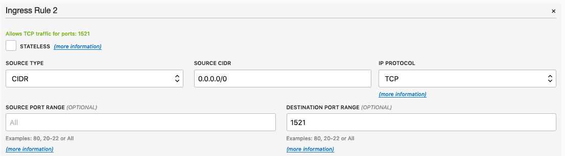
Until everything is completed. Screenshot 2019-03-04 11.01.40 
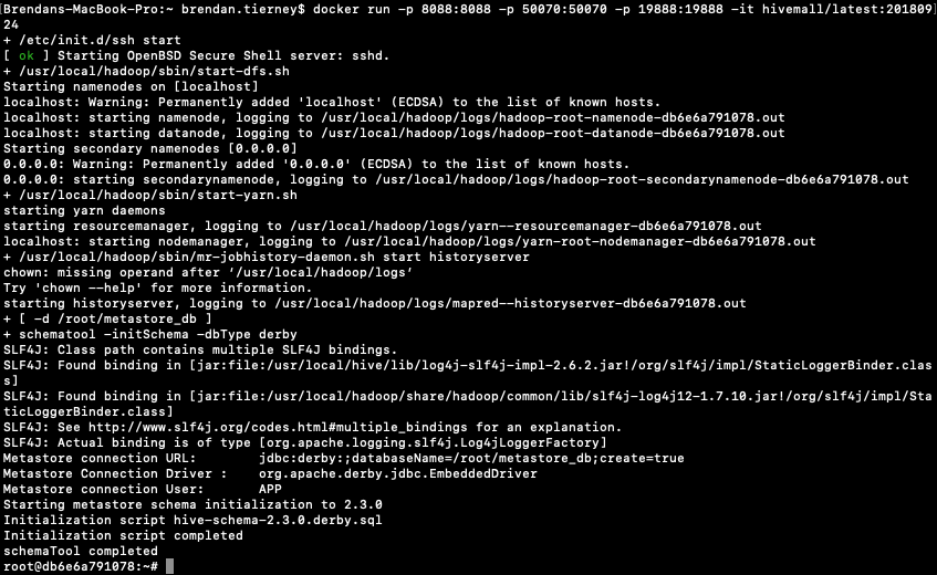
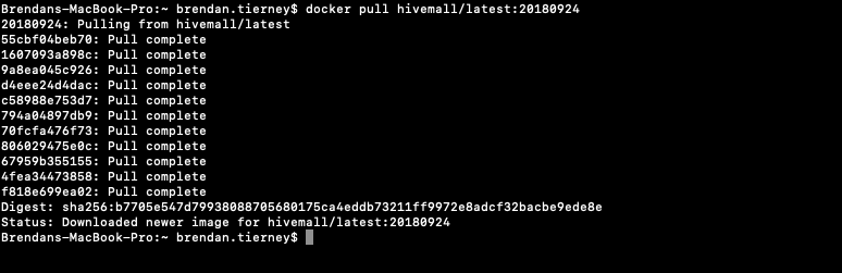
This docker image has HDFS, Yarn and MapReduce installed and running. This will require the exposing of the ports for these services 8088, 50070 and 19888. To start the HiveMall docker image run

docker run -p 8088:8088 -p 50070:50070 -p 19888:19888 -it hivemall/latest:20180924

Consider creating a shell script for this, to make it easier each time you want to run the image. Screenshot 2019-03-04 11.15.04
Now seed Hive with some data. The typical example uses the IRIS data set. Run the following command to do this. This script downloads the IRIS data set, creates a number directories and then creates an external table, in Hive, to point to the IRIS data set.
 
cd $HOME && ./bin/prepare_iris.sh
 

Screenshot 2019-03-04 11.20.49
Now open Hive and list the databases.

hive -S
hive> show databases;
OK
default
iris
Time taken: 0.131 seconds, Fetched: 2 row(s)

Connect to the IRIS database and list the tables within it.

hive> use iris;
hive> show tables;
iris_raw

Now query the data (150 records)

hive> select * from iris_raw;
1 Iris-setosa [5.1,3.5,1.4,0.2]
2 Iris-setosa [4.9,3.0,1.4,0.2]
3 Iris-setosa [4.7,3.2,1.3,0.2]
4 Iris-setosa [4.6,3.1,1.5,0.2]
5 Iris-setosa [5.0,3.6,1.4,0.2]
6 Iris-setosa [5.4,3.9,1.7,0.4]
7 Iris-setosa [4.6,3.4,1.4,0.3]
8 Iris-setosa [5.0,3.4,1.5,0.2]
9 Iris-setosa [4.4,2.9,1.4,0.2]
10 Iris-setosa [4.9,3.1,1.5,0.1]
11 Iris-setosa [5.4,3.7,1.5,0.2]
12 Iris-setosa [4.8,3.4,1.6,0.2]
13 Iris-setosa [4.8,3.0,1.4,0.1
...

Find the min and max values for each feature.

hive> select 
    > min(features[0]), max(features[0]),
    > min(features[1]), max(features[1]),
    > min(features[2]), max(features[2]),
    > min(features[3]), max(features[3])
    > from
    > iris_raw;

4.3  7.9  2.0  4.4  1.0  6.9  0.1  2.5

You are now up and running with HiveMall on Docker.

Monday, February 18, 2019

HiveML : Using SQL for ML on Big Data

It is widely recognised that SQL is one of the core languages that every data scientist needs to know. Not just know but know really well. If you are going to be working with data (big or small) you are going to use SQL to access the data. You may use some other tools and languages as part of your data science role, but for processing data SQL is king.

During the era of big data and hadoop it was all about moving the code to where the data was located. Over time we have seem a number of different languages and approaches being put forward to allow us to process the data in these big environments. One of the most common one is Spark. As with all languages there can be a large learning curve, and as newer languages become popular, the need to change and learn new languages is becoming a lot more frequent.

We have seen many of the main stream database vendors including machine learning in their databases, thereby allowing users to use machine learning using SQL. In the big data world there has been many attempts to do this, to building some SQL interfaces for machine learning in a big data environment.

One such (newer) SQL machine learning engine is called HiveMall. This will allow anyone with a basic level knowledge of SQL to quickly learn machine learning. Apache Hivemall is built to be a scalable machine learning library that runs on Apache Hive, Apache Spark, and Apache Pig.
Screenshot 2019-02-16 09.46.39

Hivemall is currently at incubator stage under Apache and version 0.6 was released in December 2018.

I've a number of big data/hadoop environments in my home lab and build on a couple of cloud vendors (Oracle and AWS). I've completed the installation of Hivemall easily on my Oracle BigDataLite VM and my own custom build Hadoop environment on Oracle cloud. A few simple commands you will have Hivemall up and running. Initially installed for just Hive and then updated to use Spark.

Hivemall expands the analytical functions available in Hive, as well as providing data preparation and the typical range of machine learning functions that are necessary for 97+% of all machine learning use cases.

Download the hivemall-core-xxx-with-dependencies.jar file
 
# Setup Your Environment $HOME/.hiverc
add jar /home/myui/tmp/hivemall-core-xxx-with-dependencies.jar; 
source /home/myui/tmp/define-all.hive;

This automatically loads all Hivemall functions every time you start a Hive session
 
# Create a directory in HDFS for the JAR 
hadoop fs -mkdir -p /apps/hivemall 
hdfs dfs -chmod -R 777 /apps/hivemall 
cp hivemall-core-0.4.2-rc.2-with-dependencies.jar hivemall-with-dependencies.jar 
hdfs dfs -put hivemall-with-dependencies.jar /apps/hivemall/ 
hdfs dfs -put hivemall-with-dependencies.jar /apps/hive/warehouse

You might want to create a new DB in Hive for your Hivemall work.
 
CREATE DATABASE IF NOT EXISTS hivemall;
USE hivemall;
Then list all the Hivemall functions
show functions "hivemall.*";

+-----------------------------------------+--+
| tab_name                                |
+-----------------------------------------+--+
| hivemall.add_bias                       |
| hivemall.add_feature_index              |
| hivemall.amplify                        |
| hivemall.angular_distance               |
| hivemall.angular_similarity             |
...

Hivemall for ML using SQL is now up and running. Next step is to do try out the various analytical and ML functions.

Thursday, February 7, 2019

Ethics in the AI, Machine Learning, Data Science, etc Era

Ethics is one of those topics that everyone has a slightly different definition or view of what it means. The Oxford english dictionary defines ethics as, 'Moral principles that govern a person's behaviour or the conducting of an activity'.

As you can imagine this topic can be difficult to discuss and has many, many different aspects.

In the era of AI, Machine Learning, Data Science, etc the topic of Ethics is finally becoming an important topic. Again there are many perspective on this. I'm not going to get into these in this blog post, because if I did I could end up writing a PhD dissertation on it. 

But if you do work in the area of AI, Machine Learning, Data Science, etc you do need to think about the ethical aspects of what you do. For most people, you will be working on topics where ethics doesn't really apply. For example, examining log data, looking for trends, etc

But when you start working of projects examining individuals and their behaviours then you do need to examine the ethical aspects of such work. Everyday we experience adverts, web sites, marketing, etc that has used AI, Machine Learning and Data Science to delivery certain product offerings to us.

Just because we can do something, doesn't mean we should do it.

One particular area that I will not work on is Location Based Advertising. Imagine walking down a typical high street with lots and lots of retail stores. Your phone vibrates and on the screen there is a message. The message is a special offer or promotion for one of the shops a short distance ahead of you. You are being analysed. Your previous buying patterns and behaviours are being analysed, Your location and direction of travel is being analysed. Some one, or many AI applications are watching you. This is not anything new and there are lots of examples of this from around the world.
But what if this kind of Location Based Advertising was taken to another level. What if the shops had cameras that monitored the people walking up and down the street. What if those cameras were analysing you, analysing what clothes you are wearing, analysing the brands you are wearing, analysing what accessories you have, analysing your body language, etc. They are trying to analyse if you are the kind of person they want to sell to. They then have staff who will come up to you, as you are walking down the street, and will have customised personalised special offers on products in their store, just for you.

See the segment between 2:00 and 4:00 in this video.  This gives you an idea of what is possible.


Are you Ok with this?

As an AI, Machine Learning, Data Science professional, are you Ok with this?

The technology exists to make this kind of Location Based Marketing possible. This will be an increasing ethical consideration over the coming years for those who work in the area of AI, Machine Learning, Data Science, etc

Just because we can, doesn't mean we should!


Monday, February 4, 2019

Machine Learning Models in Python - How long does it take

We keep hearing from people about all the computing resources needed for machine learning. Sometimes it can put people off from trying it as they will think I don't have those kind of resources.

This is another blog post in my series on 'How long does it take to create a machine learning model?'

Check out my previous blog post that used data sets containing 72K, 210K, 660K, 2M and 10M records.
There was some surprising results in those these.

In this test, I'll be using Python and SciKitLearn package to create models using the same algorithms. There are a few things to keep in mind. Firstly, although they maybe based on the same algorithms, the actual implementation of them will be different in each environment (SQL vs Python).

With using Python for machine learning, one of the challenges we have is getting access to the data. Assuming the data lives in a Database then time is needed to extract that data to the local Python environment. Secondly, when using Python you will be using a computer with significantly less computing resources than a Database server. In this test I used my laptop (MacBook Pro). Thirdly, when extracting the data from the database, what method should be used.

I've addressed these below and the Oracle Database I used was the DBaaS I used in my first experiment. This is a Database hosted on Oracle Cloud.

Extracting Data to CSV File
This kind of depends on how you do this. There are hundreds of possibilities available to you, but if you are working with an Oracle Database you will probably be using SQL Developer. I used the 'export' option to create a CSV file for each of the data sets. The following table shows how long it took for each data set.

As you can see this is an incredibly slow way of exporting this data. Like I said, there are quicker ways of doing this.

After downloading the data sets, the next step is to see how load it takes to load these CSV files into a pandas data frame in Python. The following table show the timings in seconds.


You can see that Python is very efficient at loading these data sets into a pandas data frame in my Python environment.

Extracting Data using cx_Oracle Python package
As I'll be using Python to create the models and the data exists in an Oracle Database (on Oracle Cloud), I can use the cx_Oracle package to download the data sets into my Python environment. After using the cx_Oracle package to download the data I then converted it into a pandas data frame.


You can see that using cx_Oracle to download the data is a very efficient way of accessing the data.  But if the data already exists in CSV files, then the previous method would be quicker to use.

I had the array fetch size set to 10,000.  I also experimented with smaller and larger numbers for the array fetch size, but 10,000 seemed to give a quickest results.

How long to create Machine Learning Models in Python
Now we get onto checking out the timings of how long it takes to create a number of machine learning models using different algorithms and using the default settings. The algorithms include Naive Bayes, Decision Tree, GLM, SVM and Neural Networks.


I had to stop including SVM in the tests as it was taking way too long to run. For example I killed the SVM model build on the 210K data set after it was running for 5 hours.

The Neural Network models created had 3 hidden layers.

In addition to creating the models, there was some minor data preparation steps performed including factorizing, normalization and one-hot-coding. This data preparation would be comparable to the automatic data preparation steps performed by Oracle, although Oracle Automatic Data Preparation does a bit of extra work.


At the point I would encourage you to look back at my previous blog posts on timings using Oracle DBaaS and ADW.  You will see that Python, in these test cases, was quicker at creating the machine learning models. But with Python the data needed to be extracted from the database and that can take time!

A separate consideration is being able to deploy the models. The time it takes to build models is perhaps not the main consideration. You need to consider ease of deployment and use of the models.