Tuesday, April 18, 2017

ODM Model View Details Views in Oracle 12.2

A new feature for Oracle Data Mining in Oracle 12.2 is the new Model Details views.

In Oracle 11.2.0.3 and up to Oracle 12.1 you needed to use a range of PL/SQL functions (in DBMS_DATA_MINING package) to inspect the details of a data mining/machine learning model using SQL.

Check out these previous blog posts for some examples of how to use and extract model details in Oracle 12.1 and earlier versions of the database

Association Rules in ODM-Part 3

Extracting the rules from an ODM Decision Tree model

Cluster Details

Viewing Decision Tree Details

Instead of these functions there are now a lot of DB views available to inspect the details of a model. The following table summarises these various DB Views. Check out the DB views I've listed after the table, as these views might some some of the ones you might end up using most often.

I've now chance of remembering all of these and this table is a quick reference for me to find the DB views I need to use. The naming method used is very confusing but I'm sure in time I'll get the hang of them.

NOTE: For the DB Views I've listed in the following table, you will need to append the name of the ODM model to the view prefix that is listed in the table.

Data Mining Type Algorithm & Model Details 12.2 DB View Description
Association Association Rules DM$VR generated rules for Association Rules
Frequent Itemsets DM$VI describes the frequent itemsets
Transaction Itemsets DM$VT describes the transactional itemsets view
Transactional Rules DM$VA describes the transactional rule view and transactional itemsets
Classification (General views for Classification models) DM$VT

DM$VC

describes the target distribution for Classification models

describes the scoring cost matrix for Classification models

Decision Tree DM$VP

DM$VI

DM$VO

DM$VM

describes the DT hierarchy & the split info for each level in DT

describes the statistics associated with individual tree nodes

Higher level node description

describes the cost matrix used by the Decision Tree build

Generalized Linear Model DM$VD

DM$VA

describes model info for Linear Regres & Logistic Regres

describes row level info for Linear Regres & Logistic Regres

Naive Bayes DM$VP

DM$VV

describes the priors of the targets for Naïve Bayes

describes the conditional probabilities of Naïve Bayes model

Support Vector Machine DM$VL describes the coefficients of a linear SVM algorithm
Regression ??? Doe 80 50
Clustering (General views for Clustering models) DM$VD

DM$VA

DM$VH

DM$VR

Cluster model description

Cluster attribute statistics

Cluster historgram statistics

Cluster Rule statistics

k-Means DM$VD

DM$VA

DM$VH

DM$VR

k-Means model description

k-Means attribute statistics

k-Means historgram statistics

k-Means Rule statistics

O-Cluster DM$VD

DM$VA

DM$VH

DM$VR

O-Cluster model description

O-Cluster attribute statistics

O-Cluster historgram statistics

O-Cluster Rule statistics

Expectation Minimization DM$VO

DM$VB

DM$VI

DM$VF

DM$VM

DM$VP


describes the EM components

the pairwise Kullback–Leibler divergence

attribute ranking similar to that of Attribute Importance

parameters of multi-valued Bernoulli distributions

mean & variance parameters for attributes by Gaussian distribution

the coefficients used by random projections to map nested columns to a lower dimensional space

Feature Extraction Non-negative Matrix Factorization DM$VE

DM$VI

Encoding (H) of a NNMF model

H inverse matrix for NNMF model

Singular Value Decomposition DM$VE

DM$VV

DM$VU

Associated PCA information for both classes of models

describes the right-singular vectors of SVD model

describes the left-singular vectors of a SVD model

Explicit Semantic Analysis DM$VA

DM$VF

ESA attribute statistics

ESA model features

Feature Section Minimum Description Length DM$VA describes the Attribute Importance as well as the Attribute Importance rank

Normalizing and Error Handling views created by ODM Automatic Data Processing (ADP)

  • DM$VN : Normalization and Missing Value Handling
  • DM$VB : Binning

Global Model Views

  • DM$VG : Model global statistics
  • DM$VS : Computed model settings
  • DM$VW :Alerts issued during model creation

Each one of these new DB views needs their own blog post to explain what informations is being explained in each. I'm sure over time I will get round to most of these.

Monday, April 3, 2017

Managing memory allocation for Oracle R Enterprise Embedded Execution

When working with Oracle R Enterprise and particularly when you are using the ORE functions that can spawn multiple R processes, on the DB Server, you need to be very aware of the amount of memory that will be consumed for each call of the ORE function.

ORE has two sets of parallel functions for running your user defined R scripts stored in the database, as part of the Embedded R Execution feature of ORE. The R functions are called ore.groupApply, ore.rowApply and ore.indexApply. When using SQL there are "rqGroupApply" and rqRowApply. (There is no SQL function equivalent of the R function ore.indexApply)

For each parallel R process that is spawned on the DB server a certain amount of memory (RAM) will be allocated to this R process. The default size of memory to be allocated can be found by using the following query.

select name, value from sys.rq_config;

NAME                                VALUE
----------------------------------- -----------------------------------
VERSION                             1.5
MIN_VSIZE                           32M
MAX_VSIZE                           4G
MIN_NSIZE                           2M
MAX_NSIZE                           20M

The memory allocation is broken out into the amount of memory allocated for Cells and NCells for each R process.

If your parallel ORE function create a large number of parallel R processes then you can see that the amount of overall memory consumed can be significant. I've seen a few customers who very quickly run out of memory on their DB servers. Now that is something you do not want to happen.

How can you prevent this from happening ?

There are a few things you need to keep in mind when using the parallel enabled ORE functions. The first one is, how many R processes will be spawned. For most cases this can be estimated or calculated to a high degree of accuracy. Secondly, how much memory will be used to process each of the R processes. Thirdly, how memory do you have available on the DB server. Fourthly, how many other people will be running parallel R processes at the same time?

Examining and answering each of these may look to be a relatively trivial task, but the complexity behind these can increase dramatically depending on the answer to the fourth point/question above.

To calculate the amount of memory used during the ORE user defined R script, you can use the R garbage function to calculate the memory usage at the start and at the end of the R script, and then return the calculated amount. Yes you need to add this extra code to your R script and then remove it when you have calculated the memory usage.

gc.start <- gc(reset=TRUE)
...
gc.end <- gc()
gc.used <- gc.end[,7] - gc.start[,7] # amount consumed by the processing

Using this information and the answers to the points/questions I listed above you can now look at calculating how much memory you need to allocated to the R processes. You can set this to be static for all R processes or you can use some code to allocate the amount of memory that is needed for each R process. But this starts to become messy. The following gives some examples (using R) of changing the R memory allocations in the Oracle Database. Similar commands can be issued using SQL.

> sys.rqconfigset('MIN_VSIZE', '10M') -- min heap 10MB, default 32MB
> sys.rqconfigset('MAX_VSIZE', '100M') -- max heap 100MB, default 4GB
> sys.rqconfigset('MIN_NSIZE', '500K') -- min number cons cells 500x1024, default 1M
> sys.rqconfigset('MAX_NSIZE', '2M') -- max number cons cells 2M, default 20M

Some guidelines - as with all guidelines you have to consider all the other requirements for the Database, and in reality you will have to try to find a balance between what is listed here and what is actually possible.

  • Set parallel_degree_policy to MANUAL.
  • Set parallel_min_servers to the number of parallel slave processes to be started when the database instances start, this avoids start up time for the R processes. This is not a problem for long running processes. But can save time with processes running for 10s seconds
  • To avoid overloading the CPUs if the parallel_max_servers limit is reached, set the hidden parameter _parallel_statement_queuing to TRUE. Avoids overloading and lets processes wait.
  • Set application tables and their indexes to DOP 1 to reinforce the ability of ORE to determine when to use parallelism.

Understanding the memory requirements for your ORE processes can be tricky business and can take some time to work out the right balance between what is needed by the spawned parallel R processes and everything else that is going on in the Database. There will be a lot of trial and error in working this out and it is always good to reach out for some help. If you have a similar scenario and need some help or guidance let me know.

Wednesday, March 29, 2017

OUG Ireland 2017 Presentation

Here are the slides from my presentation at OUG Ireland 2017. All about running R using SQL.

Friday, March 3, 2017

Blog posts on Oracle Advanced Analytics features in 12.2

A couple of days ago Oracle finally provided us with an on-premises download for Oracle 12.2 Database.

Go and download load it from here

or

Download the Database App Development VM with 12.2 (This is what I did)

Over the past couple of months I've been using the DBaaS of 12.2, trying out some of the new Advanced Analytics option new features, and other new features. Here are the links to the blog posts on these new 12.2 new features. There will be more coming over the next few months.

New OAA features in Oracle 12.2 Database

Explicit Semantic Analysis in Oracle 12.2c Database

Explicit Semantic Analysis setup using SQL and PL/SQL

and slightly related is the new SQL Developer 4.2

Oracle Data Miner 4.2 New Features

Monday, February 13, 2017

Join the Oracle Scene Editorial Team

Are you a member of UKOUG?

How would you like to join the editorial team of Oracle Scene magazine as a deputy editor?

If you are interested we are looking to recruit 1 deputy editor to cover the Applications area and 2 deputy editors to cover the Tech area (DBA, Developer, BA, etc)

How much time is required? about 4 hours per edition, or maybe less.

What does a deputy editor do?

As part of the editorial team you will be expected to:

- Article Review

Articles submitted are uploaded to the review panel on Basecamp. During this time the editors should become familiar with the articles and have an idea of which ones would be appropriate for publication. Time approx 1.5hrs over a 2 week period.

- Editorial Call

After the review period has closed the editors come together for an editorial call (approx 1hr) to go through the feedback received on the articles, it is the editors job to validate any comments and select which articles should be chosen for publication. Time approx 1hr.

Some articles may need further rework by the authors and the editors provide comments & instructions as to the amends needed, in some cases the editors will take on the amends themselves or if they hold the relationship with the author they may wish to approach them direct. If any articles have been held over from the previous edition, the editors will relook at the articles and if any of the content needs to be updated they will advise. If we do not have articles submitted at this stage so the editors may need to source some additional content.

- Editorial Review

Once the selected articles are edited they are passed to the designer for layout, editors will then receive a first copy of the magazine where they will read the articles relevant to them (Apps or Tech) marking up on the pdf any errors in the text or images found. We try to build in time over a weekend for this with the comments due by 9am on the Monday. This is generally the last time the editors see the magazine, the next time being the digital version. Time approx 2hrs.

- Promotion

When the digital version is ready to be sent out – the editors & review panel are notified to help raise awareness of the magazine among their network.

- Article Sourcing

Call for articles is open all year as we will just hold those submitted in between the planning timeline over to the next edition. If there are particular topics that we feel would make good articles the editors are expected to help source potential authors and of course if they see good presentations again encourage those speakers to turn their presentation in to text.

- Flying the flag

Throughout the year the editors are expected to positively “fly the flag” of Oracle Scene, as a volunteer this will include, at the annual conference, taking part in the community networking to encourage future authors amongst the community.

If you are interested in a deputy editor role then submit your application now.

NewImage

Check out UKOUG webpage for more details.

Monday, January 30, 2017

Slides from the OUG Ireland meet-ups

I've finally gotten the time (and the permissions from the presenters) to make the slides from the first two OUG Ireland meet-ups available.

I've posted them on SlideShare and I've embedded them in this blog post too.


Thursday, January 26, 2017

Formatting results from ORE script in a SELECT statement

This blog post looks at how to format the output or the returned returns from an Oracle R Enterprise (ORE), user defined R function, that is run using a SELECT statement in SQL.

Sometimes this can be a bit of a challenge to work out, but it can be relatively easy once you have figured out how to do it. The following examples works through some scenarios of different results sets from a user defined R function that is stored in the Oracle Database.

To run that user defined R function using a SELECT statement I can use one of the following ORE SQL functions.

  • rqEval
  • rqTableEval
  • "rqGroupEval"
  • rqRowEval

For simplicity we will just use the first of these ORE SQL functions to illustrate the problem and how to go about solving it. The rqEval ORE SQL function is a generate purpose function to call a user defined R script stored in the database. The function does not require any input data set and but it will return some data. You could use this to generate some dummy/test data or to find some information in the database. Here is noddy example that returns my name.

BEGIN
   --sys.rqScriptDrop('GET_NAME');
   sys.rqScriptCreate('GET_NAME',
      'function() {
         res<-data.frame("Brendan")
         res
         } ');
END;

To call this user defined R function I can use the following SQL.

select *
from table(rqEval(null,
                  'select cast(''a'' as varchar2(50))  from dual',
                  'GET_NAME') );  

For text strings returned you need to cast the returned value giving a size.

If we have a numeric value being returned we can don't have to use the cast and instead use '1' as shown in the following example. This second example extends our user defined R function to return my name and a number.

BEGIN
   sys.rqScriptDrop('GET_NAME');
   sys.rqScriptCreate('GET_NAME',
      'function() {
         res<-data.frame(NAME="Brendan", YEAR=2017)
         res
         } ');
END;

To call the updated GET_NAME function we now have to process two returned columns. The first is the character string and the second is a numeric.

select *
from table(rqEval(null,
                  'select cast(''a'' as varchar2(50)) as "NAME", 1 AS YEAR  from dual',
                  'GET_NAME') );                  

These example illustrate how you can process character strings and numerics being returned by the user defined R script.

The key to setting up the format of the returned values is knowing the structure of the data frame being returned by the user defined R script. Once you know that the rest is (in theory) easy.

Monday, January 23, 2017

Oracle Data Miner 4.2 New Features

Oracle Data Miner 4.2 (part of SQL Developer 4.2) got released as an Early Adopter versions (EA) a few weeks ago.

I had an earlier blog post that looked that the new Oracle Advanced Analytics in-database new features with the Oracle 12.2 Database.

With the new/updated Oracle Data Miner (ODMr) there are a number of new features. These can be categories as 1) features all ODMr users can use now, 2) New features that are only usable when using Oracle 12.2 Database, and 3) Updates to existing algorithms that have been exposed via the ODMr tool.

The following is a round up of the main new features you can enjoy as part of ODMr 4.2 (mainly covering points 1 and 2 above)

  • You can now schedule workflows to run based on a defined schedule
  • Support for additional data types (RAW, ROWID, UROWID, URITYPE)
  • Better support for processing JSON data in the JSON Query node
  • Additional insights are displayed as part of the Model Details View
  • Additional alert monitoring and reporting
  • Better support for processing in-memory data
  • A new R Model node that allows you to include in-database ORE user defined R function to support model build, model testing and applying of new model.
  • New Explicit Semantic Analysis node (Explicit Feature Extraction)
  • New Feature Compare and Test nodes
  • New workflow status profiling perfoance improvements
  • Refresh the input data definition in nodes
  • Attribute Filter node now allows for unsupervised attribute importance ranking
  • The ability to build Partitioned data mining models

Look out for the blog posts on most of these new features over the coming months.

WARNING: Most of these new features requires an Oracle 12.2 Database.

NewImage

Monday, January 16, 2017

Explicit Semantic Analysis setup using SQL and PL/SQL

In my previous blog post I introduced the new Explicit Semantic Analysis (ESA) algorithm and gave an example of how you can build an ESA model and use it. Check out this link for that blog post.

In this blog post I will show you how you can manually create an ESA model. The reason that I'm showing you this way is that the workflow (in ODMr and it's scheduler) may not be for everyone. You may want to automate the creation or recreation of the ESA model from time to time based on certain business requirements.

In my previous blog post I showed how you can setup a training data set. This comes with ODMr 4.2 but you may need to expand this data set or to use an alternative data set that is more in keeping with your domain.

Setup the ODM Settings table

As with all ODM algorithms we need to create a settings table. This settings table allows us to store the various parameters and their values, that will be used by the algorithm.

-- Create the settings table
CREATE TABLE ESA_settings (
    setting_name VARCHAR2(30),
    setting_value VARCHAR2(30));

-- Populate the settings table
-- Specify ESA. By default, Naive Bayes is used for classification.
-- Specify ADP. By default, ADP is not used. Need to turn this on.
BEGIN
    INSERT INTO ESA_settings (setting_name, setting_value)
    VALUES (dbms_data_mining.algo_name,       
           dbms_data_mining.algo_explicit_semantic_analys);
   
    INSERT INTO ESA_settings (setting_name, setting_value)
    VALUES (dbms_data_mining.prep_auto,dbms_data_mining.prep_auto_on);
  
    INSERT INTO ESA_settings (setting_name, setting_value)
    VALUES (odms_sampling,odms_sampling_disable);
  
    commit;
END; 

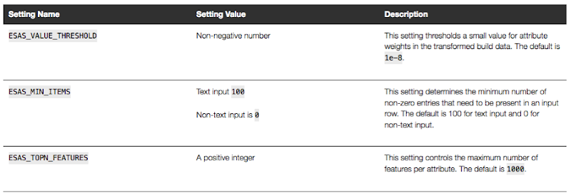
These are the minimum number of parameter setting needed to run the ESA algorithm. The other ESA algorithm setting include:

NewImage

Setup the Oracle Text Policy

You also need to setup an Oracle Text Policy and a lexer for the Stopwords.

DECLARE
   v_policy_name  varchar2(30);
   v_lexer_name   varchar2(3)
BEGIN
    v_policy_name  := 'ESA_TEXT_POLICY';
    v_lexer_name   := 'ESA_LEXER';
    ctx_ddl.create_preference(v_lexer_name, 'BASIC_LEXER');
    v_stoplist_name := 'CTXSYS.DEFAULT_STOPLIST';  -- default stop list
    ctx_ddl.create_policy(policy_name => v_policy_name, lexer => v_lexer_name, stoplist => v_stoplist_name);
END;

Create the ESA model

Once we have the settings table created with the parameter values set for the algorithm and the Oracle Text policy created, we can now create the model.

To ensure that the Oracle Text Policy is applied to the text we want to analyse we need to create a transformation list and add the Text Policy to it.

We can then pass the text transformation list as a parameter to the CREATE_MODEL, procedure.

DECLARE
   v_xlst              dbms_data_mining_transform.TRANSFORM_LIST;
   v_policy_name       VARCHAR2(130) := 'ESA_TEXT_POLICY';
   v_model_name        varchar2(50) := 'ESA_MODEL_DEMO_2';
BEGIN
   v_xlst := dbms_data_mining_transform.TRANSFORM_LIST();
   DBMS_DATA_MINING_TRANSFORM.SET_TRANSFORM(v_xlst, '"TEXT"', NULL, '"TEXT"', '"TEXT"', 'TEXT(POLICY_NAME:'||v_policy_name||')(MAX_FEATURES:3000)(MIN_DOCUMENTS:1)(TOKEN_TYPE:NORMAL)');

    DBMS_DATA_MINING.DROP_MODEL(v_model_name, TRUE);
    DBMS_DATA_MINING.CREATE_MODEL(
        model_name          => v_model_name,
        mining_function     => DBMS_DATA_MINING.FEATURE_EXTRACTION,
        data_table_name     => 'WIKISAMPLE',
        case_id_column_name => 'TITLE',
        target_column_name  => NULL,
        settings_table_name => 'ESA_SETTINGS',
        xform_list          => v_xlst);
END;

NOTE: Yes we could have merged all of the above code into one PL/SQL block.

Use the ESA model

We can now use the FEATURE_COMPARE function to use the model we just created, just like I did in my previous blog post.
SELECT FEATURE_COMPARE(ESA_MODEL_DEMO_2
               USING 'Oracle Database is the best available for managing your data' text 
               AND USING 'The SQL language is the one language that all databases have in common' text) similarity 
FROM DUAL;

Go give the ESA algorithm a go and see where you could apply it within your applications.

Monday, January 9, 2017

next OUG Ireland Meet-up on 12th January

NewImage
Our next OUG Ireland Meet-up with be on Thursday 12th January, 2017.
The theme for this meet up is DevOps and How to Migrate to the Cloud.
Come along on the night here about these topics and how companies in Ireland are doing these things.
Venue : Bank of Ireland, Grand Canal Dock, Dublin.
The agenda for the meet-up is:
18:00-18:20 Sign-in, meet and greet, networking, grab some refreshments, etc
18:20-18:30 : Introductions & Welcome, Agenda, what is OUG Ireland, etc.
18:30-19:00 : Dev Ops and Oracle PL/SQL development - Alan McClean
Abstract
In recent years the need to deliver changes to production as soon as possible has led to the rise of continuous delivery; continuous integration and continuous deployment. These issues have become standards in the application development, particularly for code developed in languages such as Java. However, database development has lagged behind in supporting this paradigm. There are a number of steps that can be taken to address this. This presentation examines how database changes can be delivered in a similar manner to other languages. The presentation will look at unit testing frameworks, code reviews and code quality as well as tools for managing database deployment.
19:00-1930 : Simplifying the journey to Oracle Cloud : Decision makers across Managers, DBA’s and Cloud Architects who need to progress an Oracle Cloud Engagement in the organization - Ken MacMahon, Head of Oracle Cloud Services at Version1
Abstract
The presentation will cover the 5 steps that Version 1 use to try and help customers with Oracle Cloud adoption in the organisation. By attending you will hear, how to deal with cloud adoption concerns, choose candidates for cloud migration, how to design the cloud architecture, how to use automation and agility in your Cloud adoption plans, and finally how to manage your Cloud environment.

This event is open to all, you don't have to be a member of the user group and best of all it is a free event. So spread the word with all your Oracle developer, DBAs, architects, data warehousing, data vizualisations, etc people.
We hope you can make it! and don't forget to register for the event.
NewImage

Wednesday, January 4, 2017

Explicit Semantic Analysis in Oracle 12.2c Database

A new Oracle Data Mining algorithm in the Oracle 12.2c Database is called Explicit Semantic Analysis.

[The following examples are built using Oracle Data Miner 4.2 (SQL Developer 4.2) and the Oracle 12.2 Database cloud service (extreme edition) ]

The Explicit Semantic Analysis algorithm is an unsupervised algorithm used for feature extraction. ESA does not discover latent features but instead uses explicit features based on an existing knowledge base. There is no setup or install necessary to use this algorithm All you need is a licence for the Advanced Analytics Option for the database. The out from the algorithm is a distance measure that indicates how similar or dis-similar the input texts are, using the ESA model (and the training data set used). Let us look at an example. Setup training data for ESA Algorithm

Oracle Data Miner 4.2 (that comes with SQL Developer 4.2) has a data Wiki data set from 2005. This contains over 200,000 features. To locate the file go to.

...\sqldeveloper\dataminer\scripts\instWikiSampleData.sql

This file contains the DDL and the insert statements for the Wiki data set.

NewImage

After you run this script a new table called WIKISAMPLE table exists and contains records

NewImage

This gives us the base/seed data set to feed into the ESA algorithm.

Create the ESA Model using ODMr

To create the ESA model we have 2 ways of doing this. In this blog post I'll show you the easiest way by using the Oracle Data Miner (ODMr) tool. I'll have another blog post that will show you the SQL needed to create the model.

In an ODMr workflow create a new Data Source node. Then set this node to have the WIKISAMPLE table as it's data source.

Next you need to create the ESA node on the workflow. This node can be found in the Models section, of the Workflow Editor. The node is called Explicit Feature Extraction. Click on this node, in the model section, and then move your mouse to your workflow and click again. The ESA node will be created.

Join the Data Node to the ESA node by right clicking on the data node and then clicking on the ESA node.

Double click on the ESA node to edit the properties of the node and the algorithm.

NewImage

Explore the ESA Model and ESA Model Features

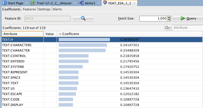
After the model node has finished you can now explore the results generated by the ESA model. Right click on the model node and select 'View Model'. The model properties window opens and it has 2 main tabs. The first of these is the coefficients tab. Here you can select a particular topic (click on the search icon beside the Feature ID) and select it from the list. The attributes and their coefficient values will be displayed.

NewImage

Next you can examine the second tab that is labeled as Features. In this table we can select a particular record and have a tag cloud and coefficients displayed. The tag cloud is a great way to see visually what words are important.

NewImage

How to use the ESA model to Compare new data using SQL

Now that we have the ESA model created, we can not use it model to compare other similar sets of documents.

You will need to use the FEATURE_COMPARE SQL function to evaluate the input texts, using the ESA model to compare for similarity. For example,

SELECT FEATURE_COMPARE(feat_esa_1_1
          USING 'Oracle Database is the best available for managing your data' text 
          AND USING 'The SQL language is the one language that all databases have in common' text) similarity 
FROM DUAL;
NewImage

The result we get is 0.7629.

The result generate by the query is a distance measure. The FEATURE_COMPARE function returns a comparison number in the range 0 to 1. Where 0 indicates that the text are not similar or related. If a 1 is returned then that indicated that the text are very similar or very related.

You can use this returned value to make a decision on what happens next. For example, it can be used to decide what the next step should be in your workflow and you can easily write application logic to manage this.

The examples given here are for general text. In the real world you would probably need a bigger data set. But if you were to use this approach in other domains, such as legal, banking, insurance, etc. then you would need to create a training data set based on the typical language that is used in each of those domains. This will then allow you to compare documents with each domain with greater accuracy.

[The above examples are built using Oracle Data Miner 4.2 (SQL Developer 4.2) and the Oracle 12.2 Database cloud service (extreme edition) ]