Monday, March 25, 2013

Review of Oracle Magazine–May/June 1999

The headline articles for the May/June 1999 edition of Oracle Magazine were focused on using internet technologies to allow businesses to work together more efficiently.

image

Other articles included:

  • Oracle and Hewlett-Packard announce the a prebuild Oralce 8i appliance. This had a code-name of Raw Iron.
  • Oracle announce a $100million venture fund to promote innovation by companies developing products and services based on Oracle 8i
  • Oracle 8i comes with the an enhanced feature that automatically keeps a standby database synchronized with the production database. This is called the Automated Standby Databases (ASD) and hopes to reduce the amount of manual work DBAs need to perform.
  • Some helpful suggestions on how to go about implementing parallel DML in Oracle 8.
    • Rules for Parallel Insert
      • The insert statement must be of the form ‘insert into table_name select …’
      • The table being modified must have a specified parallel declaration or you must specify a parallel hint directive in the insert statement
      • You can perform parallel insert on non-partitioned as well as partitioned tables
      • After the parallel DML is complete no other SQL statements can access the same table until a Commit is issued.
    • Rules for Parallel Update and Delete
      • Table table must have a parallel declaration specified or you must specify a parallel hint directive in the update/delete statement
      • You can perform parallel update or delete on partitioned tables only
      • You cannot see the result of the parallel update or delete during the transaction
  • By using the parallel options, data intensive SQL statements, database recovery, and data loads can be executed by multiple processes simultaneously. All the following operations can be executed in parallel
    • table scan
    • sort merge join
    • Not In
    • select distinct
    • aggregation
    • cube
    • create table as select
    • rebuild index partition
    • move partition
    • update
    • Insert ….. select
    • Enable constraint
    • PL/SQL functions called from SQL
    • Nested loop join
    • Hash join
    • Group by
    • Union and union all
    • Order by
    • Rollup
    • Create index
    • Rebuild index
    • Split partition
    • Delete
    • Star transformation

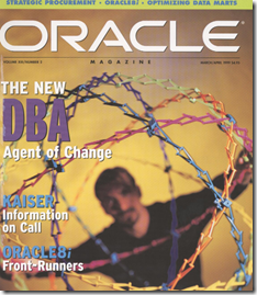
To view the cover page and the table of contents click on the image at the top of this post or click here.

My Oracle Magazine Collection can be found here. You will find links to my blog posts on previous editions and a PDF for the very first Oracle Magazine from June 1987.

Friday, March 22, 2013

Type I and Type II Data Scientists

Over the past 18 months we have seen a significant increase in the use of the term Data Scientist. Maybe it is because the HBR and many other publications have been promoting it.

Yes the areas of statistics and predictive analytics has evolved to include a lot more techniques and technologies.

Unfortunately the term Data Scientist has been over used and a lot of people have joined in with the Marketing hype. There are reports of organisations hiring a data scientist only to fire them within a few months because they did not deliver anything useful. Data Science is not some silver bullet to an organization problems and data science may not deliver anything useful, but in the vast majority of cases it will.

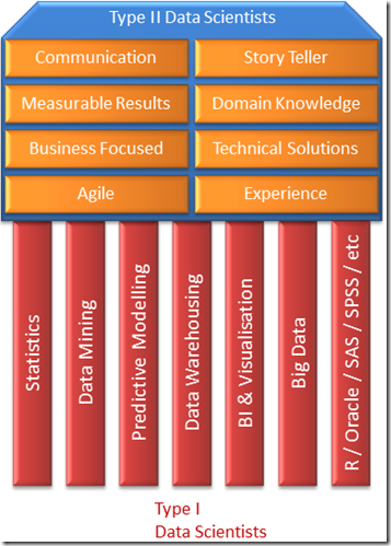
One thing that has been emerging over the past few weeks is that there seems to be two main types of Data Scientist. There are the Data Scientists who perform certain tasks or are focused on specific technologies. Then there are the Data Scientists who are not as technical as the previous group but are focused on how they can use the technologies to deliver business benefit.  I like to call these Type I and Type II Data Scientist.

The Type I Data Scientist

This is perhaps to most common type of Data Scientist we see around, or the most common type of person who is calling themselves a Data Scientist. These are people who know a lot about and are really good at a technique or technology that is associated with Data Science. Some of these would be the “old school” type of people and include:

  • Statisticians
  • Data Miners
  • Predictive Modellers
  • Machine Learning
  • Data Warehousing
  • Business Intelligence & Visualization
  • Big Data
  • R / Oracle / SAS / SPSS / etc.

The people in each of these have a deep knowledge of their topic and can tell/show you lots of detail about how best to explore data in their given field.

Yes you don’t have to have a Stats background to call yourself a Data Scientist, but some knowledge of Stats would be useful (you don’t need a PhD or Master)

The Type II Data Scientist

A Type II Data Scientist is a slightly different breed of person. They would have a little bit of knowledge of some or all of the areas listed under the Type I Data Scientist, but would not have the depth of knowledge of a topic that a Type I Data Scientist would have.

The Type II Data Scientist approaches the types of problems that organisations are facing in a different way. They will concentrate on the business goals and business problems that the organisation are facing. Based on these they will identify what the data scientist project will focus on, ensuring that there is a measurable outcome and business goal. The Type II Data Scientist will be a good communicator, being able to translate between the business problem and the technical environment necessary to deliver what is needed. During the project the data science team will discovery various insight about the data. The Type II Data Scientist will prioritise these and feed them back to the various business units. Some of these insights can range from something new, verifying business knowledge beliefs, areas where better data capture is needed, improvements in applications, etc.

The Type II Data Scientist would be the Data Science team leader within the organisation that manages the Type I Data Scientists, keeping them focused on the key deliverables of delivering measurable business benefits.

image

I really like the following phrase that I have come across recently:

“We haven't learned how to handle small data well, let alone throw big data on there.”

Data Science is not about Big Data. There is much more an organization can do with Data Science without having to get involved with Big Data. This is where the skills of the Type II Data Scientist is important, as they can direct the managers of an organization to focus on their real data problems and not get carried away with some of the marketing hype. When the time is right they will look at incorporating typical big data problems within their existing analytical environment.

One thing is for sure. The definition of “what is a” Data Scientist is still evolving. But there does seem to be some consensus the corresponds to the separation of the Type I and Type II Data Scientist roles.

Thursday, March 14, 2013

Clustering in Oracle Data Miner-Part 5

This is a the fifth and final blog post on building and using Clustering in Oracle Data Miner. The following outlines the contents of each post in this series on Clustering.

  1. The first part we looked at what clustering features exist in ODM and how to setup the data that we will be using in the examples
  2. The second part will focus on how to building Clusters in ODM .
  3. The third post will focus on examining the clusters produced by ODM and how to use the Clusters to apply to new data using ODM.
  4. The fourth post will look at how you can build and evaluate a Clustering model using the ODM SQL and PL/SQL functions.
  5. The fifth and final post will look at how you can apply your Clustering model to new data using the ODM SQL and PL/SQL functions.


Step 1 – What Clustering models do we have

In my previous post I gave the query to retrieve the clustering models that we have in our schema. Here it is again.

column model_name format a20
column mining_function format a20
column algorithm format a20
SELECT model_name,
       mining_function,
       algorithm,
       build_duration,
       model_size
FROM ALL_MINING_MODELS
WHERE mining_function = 'CLUSTERING';

image

This time we see that we have 3 cluster models. Our new model is called CLUSTER_KMEANS_MODEL.  

column child format a40
column cluster_id format a25

select cluster_id,
       record_count,
       parent,
       tree_level,
       child
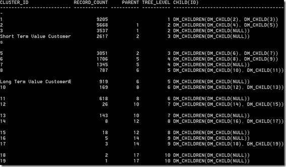
from table(dbms_data_mining.get_model_details_km('CLUS_KM_1_25'))

The following image shows all the clusters produced and we can see that we have the renamed cluster labels we set when we used the ODM tool.

image

Step 2 – Setting up the new data

There are some simple rules to consider when preparing the data for the cluster model. These really apply to all of the data mining algorithms.

- You will need to have the data prepared and in the same format as you used for building the model

- This will include the same table structure. Generally this should not be a problem. If you need to merge a number of tables to form a table with the correct format, the simplest method is to create a view.

- All the data processing for the records and each attribute needs to be completed before you run the apply function.

- Depending on the complexity of this you can either build this into the view (mentioned above), run some pl/sql procedures and create a new table with the output, etc.  I would strongly suggest that the minimum pre-processing you have to do on the data the simpler the overall process and implementation will be.

- The table or view must have one attribute for the CASE_ID. The CASE_ID is an attribute that is unique for each record. If the primary key of the table is just one attribute you can use this. If not then you will need to generate a new attribute that is unique. One way to do this is to concatenate each of the attributes that form the primary key.

Step 3 – Applying the Cluster model to new data – In Batch mode

There are two ways of using an Oracle Data Mining model in the database. In this section we will look at how you can run the cluster model to score data in a batch mode. What I mean by batch mode is that you have a table of data available and you want to score the data with what the model thinks their cluster will be.

To do this we need to run the APPLY function that is part of the DBMS_DATA_MINING package.

image

image

For clustering we do not have CASE_ID, so we can leave this parameter NULL.

One of the parameters is called RESULT_TABLE_NAME. Using the DBMS_DATA_MINING.APPLY package and function, it looks to create a new table that will contain the outputs of the cluster scoring. This table (for the KMeans and O-Cluster algorithms) will contain three attributes.

CASE_ID       VARCHAR2/NUMBER
CLUSTER_ID    NUMBER
PROBABILITY   NUMBER

The table will have the CASE_ID. This is the effectively the primary key of the table.

If we take our INSURANCE_CUST_LTV table as the table containing the new data we want to score (Yes this is the same table we used to build the cluster model) and the CLUSTER_KMEANS_MODEL as the cluster model we want to use. The following codes show the APPLY function necessary to score the data.

BEGIN  

  DBMS_DATA_MINING.APPLY(
     model_name          => 'CLUSTER_KMEANS_MODEL',
     data_table_name     => 'INSURANCE_CUST_LTV',
     case_id_column_name => 'CUSTOMER_ID',
     result_table_name   => 'CLUSTER_APPLY_RESULT');
END;

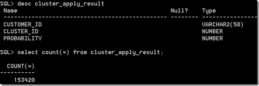
On my laptop this took 3 second to complete. This involved scoring 15,342 records, creating the table CLUSTER_APPLY_RESULT and inserting 153,420 scored records into the table CLUSTER_APPLY_RESULT.

image

Why did we get 10 times more records in our results table than we did in our source table ?

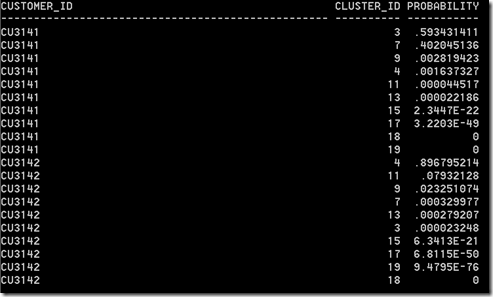
Using the batch mode i.e. using the DBMS_DATA_MINING.APPLY function it will create a record for each of the possible clusters that the record will belong too along with the probability of it belonging to that cluster. In our case we have built our clustering models based on 10 clusters.

In the following diagram we have a listing for two of the customers in our dataset, the clusters that have been assigned to them and the probability of that record/customer belonging to that cluster. We can then use this information to make various segmentation decisions based on the probabilities that each has for the various clusters.

image

Step 4 – Applying the Cluster model to new data – In Real-time mode

When we looked at applying a classification algorithm to new data we were able to use the PREDICTION SQL function. As clustering is an unsupervised data mining technique we will not be able to use the PREDICTION function.

Instead we have the functions CLUSTER_ID and CLUSTER_PROBABILITY.

CLUSTER_ID will tell us what cluster the record is most likely to belong too i.e. the cluster with the highest probability.

This is different to the bulk processing approach as we will only get one record/result being returned.

In the following example we are asking what cluster do these two customers most likely belong too.

SELECT customer_id,
       cluster_id(cluster_kmeans_model USING *) as Cluster_Num
FROM   insurance_cust_ltv
WHERE  customer_id in ('CU3141', 'CU3142');

image

Is we look back to Step 3 above we will see that the clusters listed correspond to what we have discovered.

The next function is CLUSTER_PROBABILTY. With this function we can see what the probability of customer belonging to a particular cluster. Using the results for customer CU3141 we can see what the probability is for this cluster, along with a few other clusters.

SELECT customer_id,
       cluster_probability(cluster_kmeans_model, '3' USING *) as Cluster_3_Prob,
       cluster_probability(cluster_kmeans_model, '4' USING *) as Cluster_4_Prob,
       cluster_probability(cluster_kmeans_model, '7' USING *) as Cluster_7_Prob,
       cluster_probability(cluster_kmeans_model, '9' USING *) as Cluster_9_Prob
FROM   insurance_cust_ltv
WHERE  customer_id = 'CU3141';

image

We can also combine the CLUSTER_ID and CLUSER_PROBABILITY functions in one SELECT statement.

In the following query we want to know what the most likely cluster is for two customers and the cluster probability.

SELECT customer_id,
       cluster_id(cluster_kmeans_model USING *) as Cluster_Num,
        cluster_probability(cluster_kmeans_model, cluster_id(cluster_kmeans_model USING *) USING *) as Cluster_Prob
FROM   insurance_cust_ltv
WHERE  customer_id in ('CU3141', 'CU3142');

image

Check back soon for my more blog posts on performing data mining in Oracle, using the Oracle Data Miner tool (part of SQL Developer) and the in-database SQL and PL/SQL code.

I hope you have enjoyed blog posts on Oracle Data Miner and you have found them useful. Let me know if there are specific topics you would like me to cover.

Thanks

Brendan Tierney

Monday, March 11, 2013

Oracle Magazine–March/April 1999

The headline articles for the March/April 1999 edition of Oracle Magazine were on the evolving world of the DBA. With some much new technology available in the database the role of the DBA is moving from a back office type role to one having a significant strategic influence in the organisation.
image
Other articles included:
  • Oracle releases a web based version of their Oracle Strategic Procurement application that includes three key parts: Strategic Sourcing, Internet Procurement and Process Automation.
  • Sun and Oracle announce a strategic agreement that allows both companies to enhance their product offerings by exchanging key technologies. Oracle will use the core of the Sun Solaris operating environment to deliver the industry’s first database server appliances.
  • Oracle Data Mart Suite releases version 2.5. It includes, Oracle Data Mart Builder, Oracle Data Mart Designer, Oracle 8 Enterprise Edition, Oracle Discoverer, Oracle Application Server and Oracle Reports and Reports Server.
  • New integration between Oracle Reports release 6.0 and Oracle Express Server release 6.2 to give users the ability to distribute high quality reports of information held in a multi-dimensional database across the enterprise.
  • The need for the DBA to know and understand the V$ views has been increasing during the later releases of 7.3 and 8i. The can be used for a variety of purposes, including understanding locked users, system resources, licencing and parameter settings.
  • One thing that all DBAs need to plan for is a database recovery. Planning it is one thing, but practicing it is another thing. A typical recovery plan will include, choosing a data file, create a backup, take the damaged tablespace offline, restore the damaged data file, bring the tablespace back online, recover the tablespace, bring the tablespace back online and test it.
  • Avoiding trigger errors, including Mutating and constraining table errors.
  • There is an article by Bryan Laplante on using Historgrams to Optimize Data Mart Performance.

To view the cover page and the table of contents click on the image at the top of this post or click here.
My Oracle Magazine Collection can be found here. You will find links to my blog posts on previous editions and a PDF for the very first Oracle Magazine from June 1987.

Tuesday, March 5, 2013

Clustering in Oracle Data Miner–Part 4

This is a the fourth part of a five (5) part blog post on building and using Clustering in Oracle Data Miner. The following outlines the contents of each post in this series on Clustering.
  1. The first part we looked at what clustering features exist in ODM and how to setup the data that we will be using in the examples
  2. The second part will focus on how to building Clusters in ODM .
  3. The third post will focus on examining the clusters produced by ODM and how to use the Clusters to apply to new data using ODM.
  4. The fourth post will look at how you can build and evaluate a Clustering model using the ODM SQL and PL/SQL functions.
  5. The fifth and final post will look at how you can apply your Clustering model to new data using the ODM SQL and PL/SQL functions.
With Clustering we are trying to find hidden patterns in our data. Unlike classification we a not directing the algorithms on what areas/attributes to focus on.
In my preceding post on Clustering in Oracle Data Miner I showed how you can use the Oracle Data Miner (ODM) tool, that is part of SQL Developer, to build a cluster model and to apply it to new data.
As I have shown in previous blog posts we can do all of the same steps using SQL and PL/SQL. In this blog post I will show you how to to these SQL and PL/SQL functions to generate a Clustering model and how you can evaluate the model produced.
Step 1 – What Cluster Models to we already have
Oracle Data Miner comes with a number of data dictionary tables. We can use these to see what already exists in our schema. In the example below we will have a look to see the Cluster models that were produced in the Part 2 blog post.
format model_name format a20
format mining_function format a20
format algorithm format a20

SELECT model_name,
       mining_function, 
       algorithm, 
       build_duration, 
       model_size
FROM ALL_MINING_MODELS
WHERE mining_function = 'CLUSTERING';

image
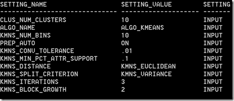
We can also look at the model settings that ODM produced. We can look at the settings of the K-Means model. This model (in my case) is called CLUS_KM_1_25.
column setting_value format a20
select setting_name,
         setting_value,
         setting_type
from  all_mining_model_settings
where model_name = 'CLUS_KM_1_25'

image
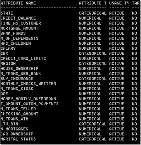
We can also look to see what attributes are used in the K-Mean model.
SELECT attribute_name, 
       attribute_type, 
       usage_type, 
       target
from  all_mining_model_attributes
where model_name = 'CLUS_KM_1_25'

image
I will show you how to use this Clustering model or the one that we are about to generate in my next blog post.
Step 2 – Creating the Setting table
When creating an Oracle Data Mining model in SQL you need to create Setting table. This will contain a record for each setting they you need to set for the algorithm you want to run. The settings table has a very basic structure and only consists of two columns. It is a good idea to create a separate Settings table for each algorithm or type of data mining you want to do. To create the settings table we run the following:
CREATE TABLE CLUSTER_SETTINGS (
Setting_Name  VARCHAR2(30),
Setting_Value VARCHAR2(4000));

The next step is to define the setting we want to use. The first of these will be the actual algorithm you want to run. Oracle has two Clustering algorithms: algo_kmeans and algo_o_cluster. In the examples we are working through we are using the K-Mean algorithm and we want to set the number of clusters to 10. We are also going to set the Automatic Data Preparation (ADP) on. Here is the code.
BEGIN
   INSERT INTO CLUSTER_SETTINGS (setting_name, setting_value)
   VALUES (dbms_data_mining.algo_name, dbms_data_mining.ALGO_KMEANS);
   INSERT INTO CLUSTER_SETTINGS (setting_name, setting_value)
   VALUES (dbms_data_mining.prep_auto, dbms_data_mining.PREP_AUTO_ON);
   INSERT INTO CLUSTER_SETTINGS (setting_name, setting_value)
   VALUES (dbms_data_mining.clus_num_clusters, 10);
  
   COMMIT;
END;

We can check to see that these records were inserted.
column setting_value format a25
select * from CLUSTER_SETTINGS;
image
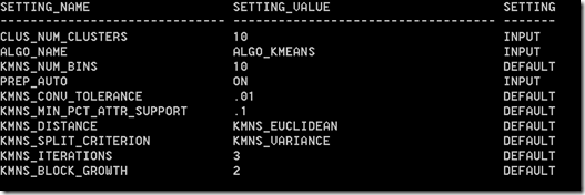
The other settings will be dependent on what clustering algorithm is being used. Each one has their own setting. If you do not define any additional setting Oracle will use the in-build default settings.
To see what the default settings:
column setting_value format a35
select *
from table(dbms_data_mining.get_default_settings)
where setting_name like 'KM%';

image
If you want to use a different value to the default, just create a new record in the CLUSTER_SETTINGS table with the new value.

Step 3 – Create the new Cluster Model
We have the algorithm settings ready, so the next steps is to create the Cluster model. We will be using the DBMS_DATA_MINING.CREATE_MODEL function and pointing it to our CLUSTER_SETTINGS table.
BEGIN
   DBMS_DATA_MINING.CREATE_MODEL(
      model_name          => 'CLUSTER_KMEANS_MODEL',
      mining_function     => dbms_data_mining.clustering,
      data_table_name     => 'INSURANCE_CUST_LTV',
      case_id_column_name => 'CUSTOMER_ID',
      target_column_name  => null,
      settings_table_name => 'CLUSTER_SETTINGS');
END;

This takes a few seconds to run on my laptop. When finished we can uses queries like we used in Step 1 above to find out the details of what was produced.
Step 4 – Examining the Cluster model
The first thing that we will need to check is that the model was created.
format model_name format a20
format mining_function format a15
format algorithm format a15

SELECT model_name, 
       mining_function,
       algorithm,
       build_duration,
       model_size
FROM ALL_MINING_MODELS
WHERE mining_function = 'CLUSTERING';

image
One thing that is a bit curious is the mode size. We have basically created two K-means models using the same settings, but the final models have different sizes. See below for an explanation.
Now lets look at the algorithms settings for our new Cluster model (Cluster KMeans Model)
select setting_name,
       setting_value,
       setting_type
from  all_mining_model_settings
where model_name = 'CLUSTER_KMEANS_MODEL'

image
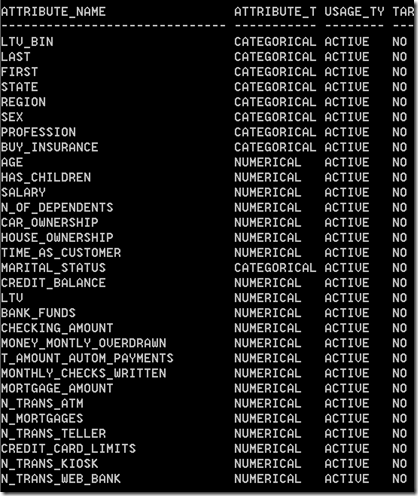
We can also look at the attributes used in the clusters.
SELECT attribute_name, 
       attribute_type, 
       usage_type, 
       target
from  all_mining_model_attributes
where model_name = 'CLUSTER_KMEANS_MODEL'
image
If we compare this list back to the list of attributes that were part of the model that we developed in the ODM tool, you will see that we have some extra attributes listed for the new K-means model.
The reason for these extra attributes and the bigger size (although still small) will be due to us having applied a sampling in the ODM tool. We took a subset of the data in the ODM tool and built the model based on this data. For the model we just created in SQL we took all the data (no sampling). That is why it would have looked at including more attributes because it was looking at a much bigger data set, etc.
Step 5 – Examining the Cluster Details
In this step we are going to look at some of the clusters produced by our new Cluster model.
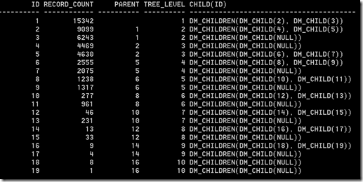
We can produce the information relating to the clusters that were produced and what level in the hierarchy each cluster belongs. We can use this information to create/draw our own cluster hierarchy diagram.
set lines 90
column child format a40

select id, 
       record_count, 
       parent, 
       tree_level, 
       child
from table(dbms_data_mining.get_model_details_km('CLUSTER_KMEANS_MODEL'))

image
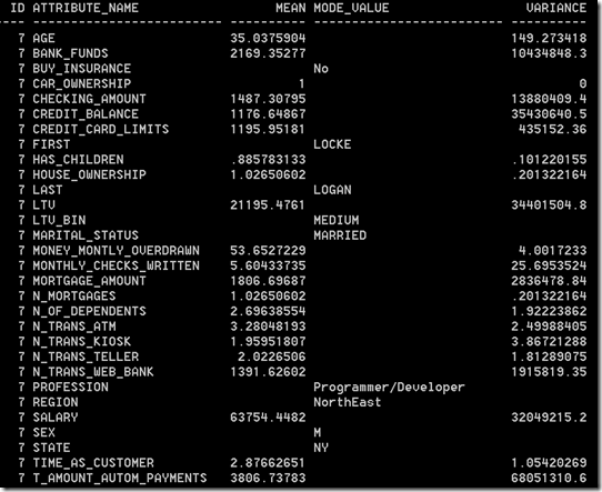
To look at the Centroid details for a particular cluster e.g. Cluster ID = 7, we can run:
column attribute_name format a25
column mode_value format a25

select t.id,
       c.attribute_name, 
       c.mean,
       c.mode_value,
       c.variance
from table (dbms_data_mining.get_model_details_KM('CLUSTER_KMEANS_MODEL')) t,
     table(t.centroid) c
where t.id = 7
order by c.attribute_name

The results will contain details of the centroid for cluster number 7. The centroid details will include the attributes that were used to form the centroid and the values for each attribute.
image
The last thing we can look at is the rule for a cluster. The following query will give you the full details of the cluster rule for Cluster 7. This will give for each attribute what the values or ranges of values that is used for that cluster. I’ll let you run this as it returns a large number of records. Run it and have a look at some of the output.
select t.id, 
       a.attribute_name, 
       a.conditional_operator,
       nvl(a.attribute_str_value,
       a.attribute_num_value) AS value,
       a.attribute_support,
       a.attribute_confidence
from TABLE(dbms_data_mining.get_model_details_km('CLUSTER_KMEANS_MODEL'))  t, 
     TABLE(t.rule.antecedent)  a
where t.id = 7
ORDER BY t.id, a.attribute_name, attribute_support, attribute_confidence desc, value;


My next blog post on Clustering in Oracle, will be the final one in the series. It will show you how to apply a Clustering model to new data in your database.

Wednesday, February 27, 2013

Clustering in Oracle Data Miner–Part 3

This is a the third part of a five (5) part blog post on building and using Clustering in Oracle Data Miner. The following outlines the contents of each post in this series on Clustering.

  1. The first part we looked at what clustering features exist in ODM and how to setup the data that we will be using in the examples
  2. The second part will focus on how to building Clusters in ODM .
  3. The third post will focus on examining the clusters produced by ODM and how to use the Clusters to apply to new data using ODM.
  4. The fourth post will look at how you can build and evaluate a Clustering model using the ODM SQL and PL/SQL functions.
  5. The fifth and final post will look at how you can apply your Clustering model to new data using the ODM SQL and PL/SQL functions.

In my previous posts on Clustering in ODM we have setup our data, we have explored it, we have taken a sample of the data and used this sample as input to the Cluster Build node. Oracle Data Miner has two clustering algorithms and our Cluster Build node created a clustering model for each.

In this post we will look at the next steps. The first of these is that we will look at examining what clustering models ODM produced. In the second part we will look at how we can use one of these clustering models to apply and label new data.
image

Step 1 – View the Cluster Models

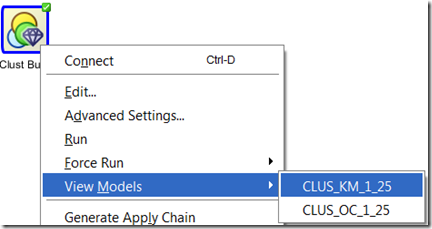
To view the the cluster modes we need to right click the Cluster Build node and select View Models from the drop down list. We get an additional down down menu that gives the names of the two cluster models that were developed.

In my case these are called CLUS_KM_1_25 and CLUS_OC_1_25. You may get different numbers on your model names. These numbers are generated internally in ODM
image

The first mode that we will look at will be the K-Mean Cluster Model (CLUS_KM_1_25). Select this from the menu.

Step 2 – View the Cluster Rules

The hierarchical K-Mean cluster mode will be displayed. You might need to readjust/resize some of the worksheets/message panes etc in ODM to get the good portion of the diagram to display.
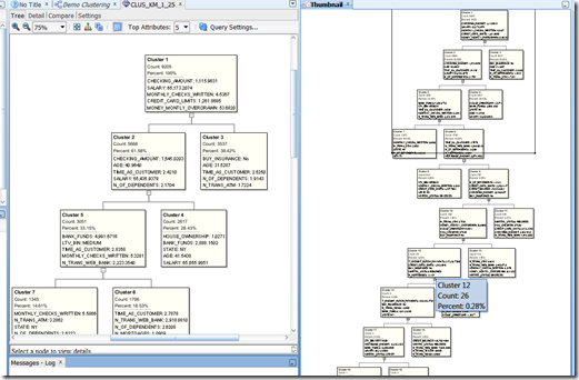
image

With ODM you cannot change, alter, merge, split, etc any the clusters that were generated. Oracle take the view of, this is what we have found it it up to you now to decide how you are going to use it.

To see that the cluster rules are for each cluster you can click on a cluster. When you do this you should get a pane (under the cluster diagram) that will contain two tabs, Centroid and Cluster Rule.

The Centroid tab provides a list of the attributes that best define the selected cluster, along with the average value for each attribute and some basic statistical information.

image

The Cluster Rules tab contains a set of rules that define the cluster in a IF/THEN statement format.
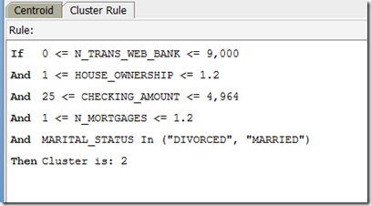
image

For each cluster in the tree we can see the number of cases in each cluster the percentage of overall cases for this cluster.

Work your way down the tree exploring each of the clusters produced.

The further down the tree you go the smaller the percentage of cases will fall into each cluster. In some tools you can merge these clusters. Not so in ODM. What you have to do is to use an IF statement in your code. Something like IF cluster_num IN (16, 17, 18, 19) THEN …..

Step 3 – Compare Clusters

In addition to the cluster tree, ODM also has two addition tabs to allow us to explore the clusters. These are Detail and Compare tabs.

image

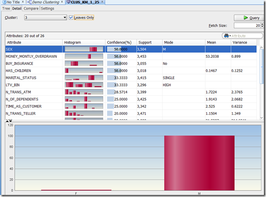
Click on the Detail tab. We now get a detailed screen that contain various statistical information for each attribute. We can for each attribute get a histogram of the values within each attribute for this cluster.

We can use this important to start building up a picture of what each cluster might represent based on the values (and their distribution) for each cluster.
image

Try this out for a few clusters.

Step 4 – Multi-Cluster - Multi-variable Comparison of Clusters

The next level of comparison and evaluation of the clusters can be found under the Compare tab.

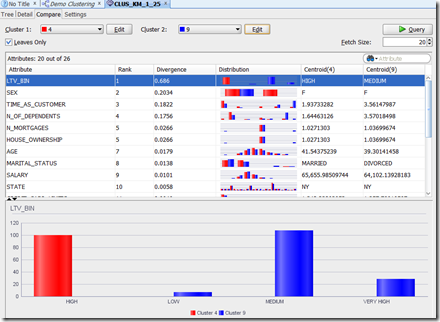
This lets us compare two clusters against each other at an attribute level. For example let us compare cluster 4 and 9. The attribute and graphics section gets updated to reflect the data for each of cluster. These are colour coded to distinguish the two clusters.
image 

We can work our way down through each attribute and again we can use this information to help us to understand what each cluster might represent.

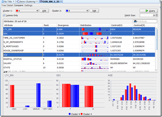
An additional feature here is that we can do multi-variable (attribute) comparison. Holding down the control button select LTV_BIN, SEX and AGE. With each selection we get a new graph appearing at the bottom of the screen. This shows the distribution of the values by attribute for each cluster.  We can learn a lot from this.
image

So one possible conclusion we could draw from this data would be that Cluster 4 could be ‘Short Term Value Customers’ and Cluster 9 could be ‘Long Term Value Customer’

Step 5 – Renaming Clusters

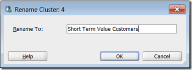
When you have discovered a possible meaning for a Cluster, you can give it a meaningful name instead of it having a number. In our example, we would like to re-label Cluster 4 to ‘Short Term Value Customers’. To do this click on the Edit button that is beside the drop down that has cluster 4. Enter the new label and click OK.
SNAGHTML1bf2277

In the drop down we will now get the new label appearing instead of the cluster number.

Similarly we can do this for the other cluster e.g. ‘Long Term Value Customer’.

image


We have just looked at how to explore our K-Means model. You can do similar exploration of the O-Cluster model. I’ll leave that for you to do.


We have now explored our clusters and we have decided which of our Clustering Models best suits our needs. In our scenario we are going to select the K-Mean model to apply and label our new data.

Step 1 – Create the Apply Node

We have already setup our sample of data that we are going to use as our Apply Data Set. We did this when we setup the two different Sample node.

We are going to use the Sample node that was set to 40%.

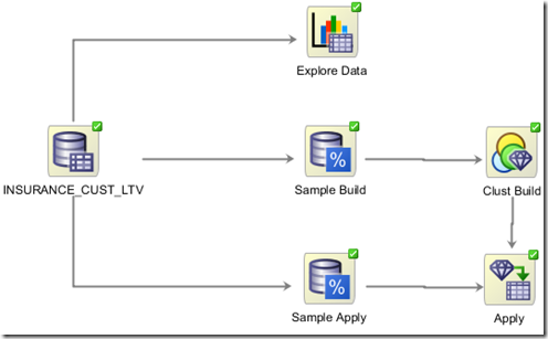
The first step requires us to create an Apply Node. This can be found under the Component Palette and Evaluate and Apply tab. Click on the Apply node and move the mouse to the workflow worksheet and click near the Sample Apply node.

To connect the two nodes, move the mouse to the Sample Apply node and right click. Select Connect from the drop down menu and then move the mouse to the Apply node and click again. An connection arrow will be created joining these nodes.

Step 2 – Specify which Clustering Model to use & Output Data

Next we need to specify which of the clustering model we want to use to apply to our new data.

We need to connect the Cluster Build node to the Apply node. Move the mouse to the Cluster Build node, right click and select connect from the drop down menu. Move the mouse to the Apply node and click. We get the connection arrow between the two node.

We now have joined the Data and the Cluster Build node to the Apply node.

The final step is to specify what clustering mode we would like to use. In our scenario we are going to specify the K-Mean model.

(Single) Click the Cluster Build node. We now need to use the Property Inspector to select the K-Means model for the apply set. In the Models tab of the Property Inspector we should have our two cluster models listed. Under the Output column click in the box for the O-Cluster model. We should now get a little red X mark appearing. The K-Mean model should still have the green arrow under the Output column.

Step 3 – Run the Apply Node

We have one last data setup to do on the Apply node. We need to specify what data from the apply data set we want to include in the output from the Apply node.  For simplicity we want to just include the primary key, but you could include all the attributes.  In addition to including the attributes from the apply data source, the Apply Node will also create some attributes based on the Cluster model we selected. In our scenario, the K-Means model will create two additional attributes. One of these will contain the Cluster ID and the other attribute will be the probability of the that cluster being valid.

To include the attributes from the source data, double click on the Apply node. This will open the Edit Apply Node window. You will see that it already contains the two attributes that will be created by the K-Mean model.

image

To add the attributes from the source data, click on the Data Columns tab and then click on the green ‘+’ symbol. For simplicity we are going to just select the CUSTOMER_ID. Click the OK button to finish.

image

Now we are ready to run the Apply node. To do this right click on the Apply Node and select Run from the drop down menu. When everything is finished you will get the little green tick mark on the top right hand corner of the Apply node.
image

Step 4 – View the Results

To view the results and the output produced by the Apply node, right click on the Apply node and select View Data from the drop down menu.

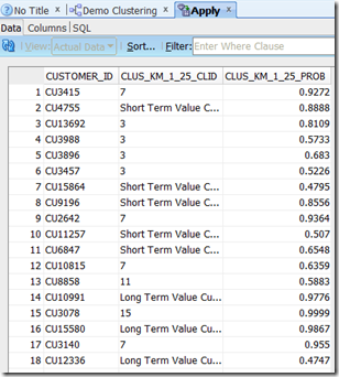
We get a new tab opened in SQL Developer that will contain the data. This will consist of the CUSTOMER_ID, the K-means Cluster ID and the Cluster Probability. You will see that the some of the clusters assigned will have a number and some will have the cluster labels that we assigned in a previous step.
image

It is now up to you to decide how you are going to use this clustering information in an operational or strategic way in your organisation.


In my next (fourth) blog post in the series on Clustering in Oracle Data Miner, I will show how you can perform similar steps, of building and evaluating clustering models, using the SQL and PL/SQL functions in the database. So we will not be using the ODM tool. We will be doing everything in SQL and SQL/PLSQL.

Tuesday, February 26, 2013

Anti-Social Wednesdays

It is about time that I got round to starting my New Years Resolution. What I’m calling it is Anti-Social Wednesdays.  What does this mean? Each Wednesday, I’m going to cut myself off from the “always on” culture of the IT World. This means I will not be turning on my email, twitter, facebook, LinkedIn, etc.  In addition to these I will also be turning off my Email, unplugging my Desk phone and turning off my mobile. These will only get turned back on or plugged back in on a Thursday morning.
Yes this will mean that anything “urgent” that comes up on a Wednesday will have to wait until I get to it on the Thursday (or Friday).

What am I going to do on my Anti-Social Wednesday? I will be concentrating on getting some work done (without all the interruptions), doing some DBA work, working of various projects, writing some blog posts or presentations, trying new products, testing new releases of software, etc.   Oracle 12c Database is coming out in a couple of weeks. Also a new release of SQL Developer 4 and a new release of Oracle Data Miner. So will be concentrating on these during March, April and May.

I will also be trying to do all of this work in new/different locations. So you will not find me at my desk (hopefully).

Now you might see some blog posts or tweets appearing from time to time on a Wednesday. All this means is that I had these scheduled to go on that day.

If you really, really, really, really need to contact me then you can work out how to do it or you will know how to do it!

Monday, February 25, 2013

Review of Oracle Magazine–Jan/Feb 1999

The headline articles for the Jan/Feb 1999 edition of Oracle Magazine were all on the Year 2000 issue (Y2K). There was lots of work for the consultancy companies around the work on this. Most of the work was not very interesting but was vital to ensure that our applications continued to work.

image

Other articles included:

  • Oracle Developer and Developer Server Release 6.0 allows for the migration of your existing applications to the Web
  • Oracle Enterprise Manager 2.0 is released. What version are we on now and how things have improved.
  • Oracle announces that it has begun a pilot program for its Business OnLine hosting service for enterprise applications. It will provide a full complement of the Oracle Applications for financials, manufacturing, distribution and HR on a subscription basis.
  • Oracle and DELL have teamed up to deliver Oracle8 databases preinstalled on the Dell PowerEdge servers. This was one of Oracle’s first attempts at a database machine/appliance.
  • Oracle 8 Data Cartridge allows you to extend the functionality available in PL/SQL with code that is available external to the database is now flexible and efficient manner. The steps involved in this included, and sample code was provided:
    • Create a relocatable library fro shared objects.
    • Create Oracle 8 objects.
    • Configure an external procedure listener to run the cartridge.
    • Configure tnsnames.ora with the extproc entry
  • How to recover a dropped table when you you only have a full OS backup of it and no export of the table.
    • Determine which tablespaces need to be restored in order to create the table to be recovered
    • Determine the file-system space requirements.
    • Build the database copy and establish the environment for the copy database
    • Export the required tables from the copy database, and import them back into the database that needs to be recovered
    • Oralce 8 comes with point in time recovery.

To view the cover page and the table of contents click on the image at the top of this post or click here.

My Oracle Magazine Collection can be found here. You will find links to my blog posts on previous editions and a PDF for the very first Oracle Magazine from June 1987.

Tuesday, February 19, 2013

Clustering in Oracle Data Miner–Part 2

This is a the second part of a five (5) part blog post on building and using Clustering in Oracle Data Miner. The following outlines the contents of each post in this series on Clustering.

  1. The first part we looked at what clustering features exist in ODM and how to setup the data that we will be using in the examples
  2. The second part will focus on how to building Clusters in ODM .
  3. The third post will focus on examining the clusters produced by ODM and how to use the Clusters to apply to new data using ODM.
  4. The fourth post will look at how you can build and evaluate a Clustering model using the ODM SQL and PL/SQL functions.
  5. The fifth and final post will look at how you can apply your Clustering model to new data using the ODM SQL and PL/SQL functions.

With Clustering we are trying to find hidden patterns in our data. Unlike classification we a not directing the algorithms on what areas/attributes to focus on.

In our scenario we want to look to see what distinct groupings or Segments that our Customer data naturally fit into. For each of these Segment Oracle Data Miner will tell us what attributes and the values of these attributes that determine if a customer belongs to one segment or another.

Step 1 - Define the Data Source

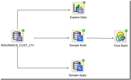
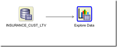
The first step involves us creating a Data Source Node for the table that we created and loaded in the previous blog post. We called this table INSURANCE_CUST_LTV.

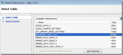
To create the Data Source Node go to the Component Palette. Under the Data tab you will find the Data Source option. Click on this and then go to the workflow worksheet and click. The Data Source node will be created and the wizard to specify the name of the table/view will open. Select INSURANCE_CUST_LTV from the list.

image

Click on the Next and then the Finish button to take in all the attribute.

Our data is now read to use.

Step 2 – Explore the Data

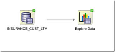
We can use the Explore Node to gather some statistics on the data and to produce some graphs.

To create the Explore Node, go to the Component Palette and under the Data tab you will find the Explore Data node. Click on this and then click again on the workflow worksheet, near the Data node.

You need to connect the Data node to the Explore Data node. Move your mouse to the Data node. Right-click this node and select Connect from the drop down menu. Then more the mouse to the Explore Data node and click on it. You will now have an arrowed line joining these two nodes

image

The next step we need to do is to right click on the Explore Data node and select Run from the drop down menu. ODM will go off to the database and gather various statistics and create a number of graphs based on the data in the table.

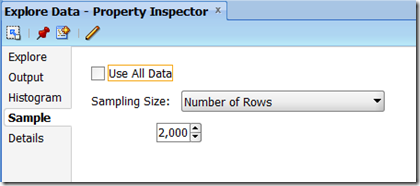
NB. If you click on the Explore Data node and then look in the Property Inspector you will see that ODM will take a sample of 2,000 records to produce the statistics and graphs. If you would like ODM to use all the records then you need to click the ‘Use All Data’ check box. Or you can change the sample size.

image

For your initial data investigation you might use the default of sampling 2,000 records before you increase the size of the sample.

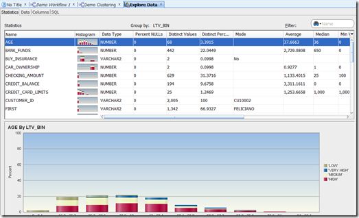
In scenarios like this you may want to explore the data in more detail and to look at how the data is distributed in relation to certain attributes. In our data we have an attribute called LTV_BIN. In this attribute we have four values including, Very High, High, Medium and Low.

In our scenario, it might be more interesting to explore the data based on this attribute and it’s values. To do this we need to tell the Explore Data node to group the data analysis based on the values in this attribute.

image

Double-click the Explore Data node. In the Group By drop down select LTV_BIN. Click the OK button. You are now ready to run the Explore Data Node. To do this, right click on Explore Data node and select Run from the drop down list.

To view the statistics gathered and the graphs produced on the default sample of 2,000 records, right click the Explore Data node and select View Data from the drop down menu. You will get a new tab/window opening in SQL Developer with all the results.

image

This kind of data analysis only works with an attribute that has a low number of possible values.

Step 3 – Defining the data we will used to Build our Cluster models

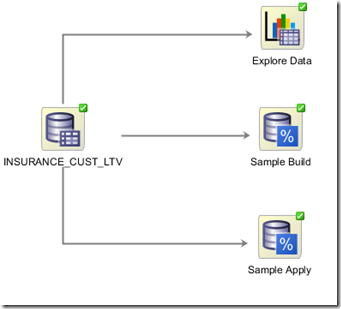
We are going to divide the data in our CUST_INSURANCE_LTV into two data sets. The first data set will be used to build the Cluster models. The second data set will be used as part of the Apply node in my next blog post (part 3).

To divide the data we are going to use the Sample Node that can be found under the Transformation tab of the Component Palette.

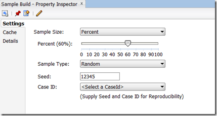
Create your first Sample Node. In the Settings tab of the Property Inspector set the sample size to 60% and in the Details tab rename the node to Sample Build.

image

Create a second Sample node and give it a sample size of 40%. Rename this node to Sample Apply.

Right click on each of these Sample nodes to run them and have them ready for the next step of building the Clustering models.

image

Step 4 – Creating the Clustering Build Node

When you have finished exploring the data you are now ready to move on to creating the Clustering models. As ODM has two clustering algorithms, ODM will default to creating two Clustering models.

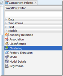
To create the Clustering models, go to the Component Palette. Under the Models tab, select Clustering.

image

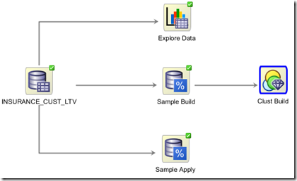
Move the mouse to the workflow worksheet, near the Sample Build node and click the worksheet. The Clustering node will be created. Now we need to connect the data with the Clustering node. To do this right click on the Sample Build node and select Connect from the drop down list. Then move the mouse to the Clustering node and click. An arrowed line will be created connecting the two nodes.

image

At this point we can run the Clustering Build node or we can have a look at the setting for each algorithm.

Step 5 – The Clustering Algorithm settings

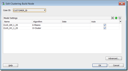
To setup the Cluster Build node you will need to double click on the node to open the properties window. The first thing that you need to do is to specify the Case ID (i.e. the primary key). In our example this is the CUSTOMER_ID.

SNAGHTML5b02a0

Oracle Data Miner has two clustering algorithms. The first of these is the well know k-Means (it is an enhanced version of it) and the O-Cluster. To look at the settings for each algorithm, click on the model listed under Model Settings and then click on the Advanced button.

A new window will open that lists all the attributes for the in the data source. The CUSTOMER_ID is unchecked as we said that this was the CASE_ID.

Click on the Algorithm Settings tab to see the internal settings for the k-means algorithm. All of these settings have a default value. Oracle has worked out what the optimal setting are for you. The main setting that you might want to play with is the Number of Clusters to build. The default is 10, but you might want to play with numbers between 5 and 15 depending on the number of clusters or segments you want to see in your data.

To view the algorithm settings for O-Cluster click on this under the Model Setting. We have less internal settings to worry about here, but we again can determine how many clusters we want to produce.

For our scenario we are going to take the default settings.

Step 6 – Run/Generate the Clustering models

At this stage we have the data set-up, the Cluster Build node created and the algorithm setting all set to what we want.

Now we are ready to run the Cluster Build node.

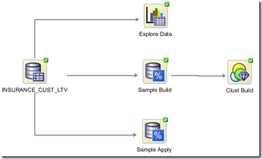
To do this, right click on the Cluster Build node and click run. ODM will go create a job that will contain PL/SQL code that will generate a cluster model based on K-Means and a second cluster model based on O-Cluster. This job will be submitted to the database and when it is completed we will get the little green tick mark on the top right hand corner of the Cluster Build node.

image


In the next blog post we will look at how to examine what clusters were produced by ODM and how we can take one of these and apply them to new data.

Wednesday, February 13, 2013

Clustering in ODM–Part 1

This is a the first part of a five (5) part blog post on building and using Clustering in Oracle Data Miner. The following outlines the contents of each post in this series on Clustering.

  1. This post part we will look at what clustering features exist in ODM and how to setup the data that we will be using in the examples
  2. The second part will focus on how to building Clusters and examining the clusters produced in ODM .
  3. The third post will focus on using the Clusters to apply to new data using ODM.
  4. The fourth post will look at how you can build and evaluate a Clustering model using the ODM SQL and PL/SQL functions.
  5. The fifth and final post will look at how you can apply your Clustering model to new data using the ODM SQL and PL/SQL functions.

Clustering is an unsupervised technique designed groupings of related data that are more similar to each other and are less similar to other groups.  Typically clustering is used in customer segmentation analysis to try an better understand what type of customers you have.

Like with all data mining techniques, Clustering will not tell you or give you some magic insight into your data. Instead it gives you more information for you to interpret and add the business meaning to them. With Clustering you can explore the data that forms each cluster to understand what it really means.

The Clusters give by Oracle Data Miner are just patterns that it has found in the data.

image

Oracle has two Clustering algorithms:

K-Means : Oracle Data Miner runs an enhanced version of the typical k-means algorithm. ODM builds models in a hierarchical manner, using a top-down approach with binary splits and refinements of all nodes at the end. The centroid of the inner nodes in the hierarchy are updated to reflect changes as the tree grows. The tree grows one node at a time. The node wit the largest variance is split to increase the size of the tree until the desired number of clusters is reached.

O-Cluster : O-Cluster is an Orthogonal Partitioning Clustering that creates a hierarchical grid based clustering model. It operates recursively, generating a hierarchical structure. The resulting clusters define dense areas.

The Data Set for out Clustering examples

I’m going to use a data set that is available on OTN (somewhere) and has been used for demos in the prior versions of ODM before the 11gR2 version (SQL Developer 3). It has gone by many names but the table name we care going to use is INSURANCE_CUST_LTV.

The file is in CSV format and we will use the Import feature in SQL Developer to import it.

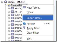
1. In the schema you are using for Oracle Data Miner, right click Tables in the Connections tab. The Import option will appear on the menu. Select this.

image

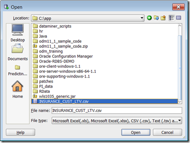
2. Go to the directory where you saved the file, select it and then click on the Open button.

SNAGHTML60a28d3

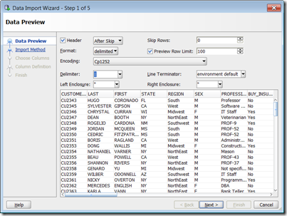
3. You need to set the file Format to be ‘Delimited’ and the Delimiter set to ‘|’

SNAGHTML60c6d04

4. In the next step give the table name as INSURANCE_CUST_LTV

5.In the next step Select all the Attributes. It should default to this. Click next.

6. In Step 4 of the Wizard you can set the data types for each attribute. The simplest way is to set the character attributes to VARCHAR2 (50) :

CUSTOMER_ID,  LAST,  FIRST,  STATE,  REGION,  SEX,  PROFESSION,  BUY_INSURANCE (set this one to 3), MARITAL_STATUS, LTV_BIN

Set all the number attributes (all the others) to NUMBER without any precision or scale.

7. Click the next button and then the finish button.  SQL Developer will now load 15,342 records into the INSURANCE_CUST_LTV table, with no errors (hopefully!)


We are now ready to start our work with the Clustering algorithms in ODM.

In the next blog post we will look at exploring the data, building our Clustering models and examining the clusters that were produced by ODM.