Monday, June 4, 2018

Twitter Analytics using Python - Part 2

This is my second (of five) post on using Python to process Twitter data.

Check out my all the posts in the series.

In this post I was going to look at two particular aspects. The first is the converting of Tweets to Pandas. This will allow you to do additional analysis of tweets. The second part of this post looks at how to setup and process streaming of tweets. The first part was longer than expected so I'm going to hold the second part for a later post.

Step 6 - Convert Tweets to Pandas

In my previous blog post I show you how to connect and download tweets. Sometimes you may want to convert these tweets into a structured format to allow you to do further analysis. A very popular way of analysing data is to us Pandas. Using Pandas to store your data is like having data stored in a spreadsheet, with columns and rows. There are also lots of analytic functions available to use with Pandas.

In my previous blog post I showed how you could extract tweets using the Twitter API and to do selective pulls using the Tweepy Python library. Now that we have these tweet how do I go about converting them into Pandas for additional analysis? But before we do that we need to understand a bit more a bout the structure of the Tweet object that is returned by the Twitter API. We can examine the structure of the User object and the Tweet object using the following commands.

dir(user)

['__class__',
 '__delattr__',
 '__dict__',
 '__dir__',
 '__doc__',
 '__eq__',
 '__format__',
 '__ge__',
 '__getattribute__',
 '__getstate__',
 '__gt__',
 '__hash__',
 '__init__',
 '__init_subclass__',
 '__le__',
 '__lt__',
 '__module__',
 '__ne__',
 '__new__',
 '__reduce__',
 '__reduce_ex__',
 '__repr__',
 '__setattr__',
 '__sizeof__',
 '__str__',
 '__subclasshook__',
 '__weakref__',
 '_api',
 '_json',
 'contributors_enabled',
 'created_at',
 'default_profile',
 'default_profile_image',
 'description',
 'entities',
 'favourites_count',
 'follow',
 'follow_request_sent',
 'followers',
 'followers_count',
 'followers_ids',
 'following',
 'friends',
 'friends_count',
 'geo_enabled',
 'has_extended_profile',
 'id',
 'id_str',
 'is_translation_enabled',
 'is_translator',
 'lang',
 'listed_count',
 'lists',
 'lists_memberships',
 'lists_subscriptions',
 'location',
 'name',
 'needs_phone_verification',
 'notifications',
 'parse',
 'parse_list',
 'profile_background_color',
 'profile_background_image_url',
 'profile_background_image_url_https',
 'profile_background_tile',
 'profile_banner_url',
 'profile_image_url',
 'profile_image_url_https',
 'profile_link_color',
 'profile_location',
 'profile_sidebar_border_color',
 'profile_sidebar_fill_color',
 'profile_text_color',
 'profile_use_background_image',
 'protected',
 'screen_name',
 'status',
 'statuses_count',
 'suspended',
 'time_zone',
 'timeline',
 'translator_type',
 'unfollow',
 'url',
 'utc_offset',
 'verified']

dir(tweets)

['__class__',
 '__delattr__',
 '__dict__',
 '__dir__',
 '__doc__',
 '__eq__',
 '__format__',
 '__ge__',
 '__getattribute__',
 '__getstate__',
 '__gt__',
 '__hash__',
 '__init__',
 '__init_subclass__',
 '__le__',
 '__lt__',
 '__module__',
 '__ne__',
 '__new__',
 '__reduce__',
 '__reduce_ex__',
 '__repr__',
 '__setattr__',
 '__sizeof__',
 '__str__',
 '__subclasshook__',
 '__weakref__',
 '_api',
 '_json',
 'author',
 'contributors',
 'coordinates',
 'created_at',
 'destroy',
 'entities',
 'favorite',
 'favorite_count',
 'favorited',
 'geo',
 'id',
 'id_str',
 'in_reply_to_screen_name',
 'in_reply_to_status_id',
 'in_reply_to_status_id_str',
 'in_reply_to_user_id',
 'in_reply_to_user_id_str',
 'is_quote_status',
 'lang',
 'parse',
 'parse_list',
 'place',
 'retweet',
 'retweet_count',
 'retweeted',
 'retweets',
 'source',
 'source_url',
 'text',
 'truncated',
 'user']

We can see all this additional information to construct what data we really want to extract.

The following example illustrates the searching for tweets containing a certain word and then extracting a subset of the metadata associated with those tweets.

oracleace_tweets = tweepy.Cursor(api.search,q="oracleace").items()
tweets_data = []
for t in oracleace_tweets:
   tweets_data.append((t.author.screen_name,
                       t.place,
                       t.lang,
                       t.created_at,
                       t.favorite_count,
                       t.retweet_count,
                       t.text.encode('utf8')))

We print the contents of the tweet_data object.

print(tweets_data)

[('jpraulji', None, 'en', datetime.datetime(2018, 5, 28, 13, 41, 59), 0, 5, 'RT @tanwanichandan: Hello Friends,\n\nODevC Yatra is schedule now for all seven location.\nThis time we have four parallel tracks i.e. Databas…'), ('opal_EPM', None, 'en', datetime.datetime(2018, 5, 28, 13, 15, 30), 0, 6, "RT @odtug: Oracle #ACE Director @CaryMillsap is presenting 2 #Kscope18 sessions you don't want to miss! \n- Hands-On Lab: How to Write Bette…"), ('msjsr', None, 'en', datetime.datetime(2018, 5, 28, 12, 32, 8), 0, 5, 'RT @tanwanichandan: Hello Friends,\n\nODevC Yatra is schedule now for all seven location.\nThis time we have four parallel tracks i.e. Databas…'), ('cmvithlani', None, 'en', datetime.datetime(2018, 5, 28, 12, 24, 10), 0, 5, 'RT @tanwanichandan: Hel ......

I've only shown a subset of the tweets_data above.

Now we want to convert the tweets_data object to a panda object. This is a relative trivial task but an important steps is to define the columns names otherwise you will end up with columns with labels 0,1,2,3...

import pandas as pd

tweets_pd = pd.DataFrame(tweets_data,
                         columns=['screen_name', 'place', 'lang', 'created_at', 'fav_count', 'retweet_count', 'text'])

Now we have a panda structure that we can use for additional analysis. This can be easily examined as follows.

tweets_pd

 	screen_name 	place 	lang 	created_at 	fav_count 	retweet_count 	text
0 	jpraulji 	None 	en 	2018-05-28 13:41:59 	0 	5 	RT @tanwanichandan: Hello Friends,\n\nODevC Ya...
1 	opal_EPM 	None 	en 	2018-05-28 13:15:30 	0 	6 	RT @odtug: Oracle #ACE Director @CaryMillsap i...
2 	msjsr 	None 	en 	2018-05-28 12:32:08 	0 	5 	RT @tanwanichandan: Hello Friends,\n\nODevC Ya...

Now we can use all the analytic features of pandas to do some analytics. For example, in the following we do a could of the number of times a language has been used in our tweets data set/panda, and then plot it.

import matplotlib.pyplot as plt

tweets_by_lang = tweets_pd['lang'].value_counts()
print(tweets_by_lang)

lang_plot = tweets_by_lang.plot(kind='bar')
lang_plot.set_xlabel("Languages")
lang_plot.set_ylabel("Num. Tweets")
lang_plot.set_title("Language Frequency")

en    182
fr      7
es      2
ca      2
et      1
in      1

Pandas1

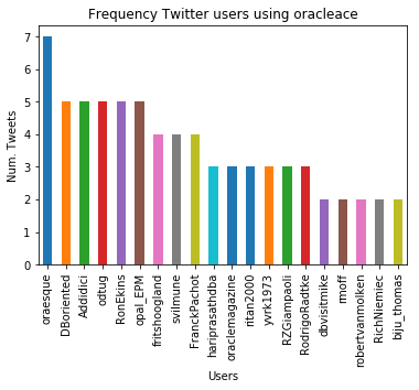
Similarly we can analyse the number of times a twitter screen name has been used, and limited to the 20 most commonly occurring screen names.

tweets_by_screen_name = tweets_pd['screen_name'].value_counts()
#print(tweets_by_screen_name)

top_twitter_screen_name = tweets_by_screen_name[:20]
print(top_twitter_screen_name)

name_plot = top_twitter_screen_name.plot(kind='bar')
name_plot.set_xlabel("Users")
name_plot.set_ylabel("Num. Tweets")
name_plot.set_title("Frequency Twitter users using oracleace")

oraesque           7
DBoriented         5
Addidici           5
odtug              5
RonEkins           5
opal_EPM           5
fritshoogland      4
svilmune           4
FranckPachot       4
hariprasathdba     3
oraclemagazine     3
ritan2000          3
yvrk1973           3
...

Pandas2

There you go, this post has shown you how to take twitter objects, convert them in pandas and then use the analytics features of pandas to aggregate the data and create some plots.


Check out the other blog posts in this series of Twitter Analytics using Python.

Wednesday, May 30, 2018

Call for Papers : UKOUG Annual Conferences : Closes 4th June at 9am (UK)

The call for Papers (presentations) for the UKOUG Annual Conferences is open until 9am (UK time) on Monday 4th June.

Ukoug18

Me: What are you waiting for? Go and submit a topic! Why not!

You: Humm, well..., (excuse, excuse, ...)

Me: What?

You: I couldn't do that! Present at a conference?

Me: Why not?

You: That is only for experts and I'm not one.

Me: Wrong! If you have a story to tell, then you can present.

You: But I've never presented before, it scares me, but one day I'd like to try.

Me: Go for it, do it. If you want you can co-present with me.

You: But, But, But .....


I'm sure you have experienced something like the above conversation before. You don't have to be an expert to present, you don't have to know everything about a product to present, you don't have to be using the latest and brightest technologies to present, you don't have to present about something complex, etc. (and the list goes on and on)

The main thing to remember is, if you have a story to tell then that is your presentation. Be it simple, complex, only you might be interested in it, it involves making lots of bits of technology work, you use a particular application in a certain way, you found something interesting, you used a new process, etc (and the list goes on and on)

I've talked to people who "ranted" for two hours about a certain topic (its was about Dates in Oracle), but when I said you should give a presentation on that, they say NO, I couldn't do that!. (If you are that person and you are reading this, then go on and submit that presentation).

If you don't want to present alone, then reach out to someone else and ask them if they are interested in co-presenting. Most experienced presenters would be very happy to do this.

You: But the topic area I'll talk about is not listed on the submission page?

Me: Good point, just submit it and pick the topic area that is closest.

You: But my topic would be of interest to the APPs and Tech conference, what do I do?

Me: Submit it to both, and let the agenda planners work out where it will fit.

I've presented at both APPs and Tech over the years and sometimess my Tech submission has been moved and accepted for the APPs conf, and vice versa.

Just do it!

Just do it

Monday, May 28, 2018

Twitter Analytics using Python - Part 1

(This is probably the first part of, probably, a five part blog series on twitter analytics using Python. Make sure to check out the other posts and I'll post a wrap up blog post that will point to all the posts in the series)

(Yes there are lots of other examples out there, but I've put these notes together as a reminder for myself and a particular project I'm testing)

In this first blog post I will look at what you need to do get get your self setup for analysing Tweets, to harvest tweets and to do some basics. These are covered in the following five steps.

Step 1 - Setup your Twitter Developer Account & Codes

Before you can start writing code you need need to get yourself setup with Twitter to allow you to download their data using the Twitter API.

To do this you need to register with Twitter. To do this go to apps.twitter.com. Log in using your twitter account if you have one. If not then you need to go create an account.

Next click on the Create New App button.

Twitter app1

Then give the Name of your app (Twitter Analytics using Python), a description, a webpage link (eg your blog or something else), click on the 'add a Callback URL' button and finally click the check box to agree with the Developer Agreement. Then click the 'Create your Twitter Application' button.

You will then get a web page like the following that contains lots of very important information. Keep the information on this page safe as you will need it later when creating your connection to Twitter.

Twitter app2

The details contained on this web page (and below what is shown in the above image) will allow you to use the Twitter REST APIs to interact with the Twitter service.

Step 2 - Install libraries for processing Twitter Data

As with most languages there is a bunch of code and libraries available for you to use. Similarly for Python and Twitter. There is the Tweepy library that is very popular. Make sure to check out the Tweepy web site for full details of what it will allow you to do.

To install Tweepy, run the following.

pip3 install tweepy

It will download and install tweepy and any dependencies.

Step 3 - Initial Python code and connecting to Twitter

You are all set to start writing Python code to access, process and analyse Tweets.

The first thing you need to do is to import the tweepy library. After that you will need to use the important codes that were defined on the Twitter webpage produced in Step 1 above, to create an authorised connection to the Twitter API.

Twitter app3

After you have filled in your consumer and access token values and run this code, you will not get any response.

Step 4 - Get User Twitter information

The easiest way to start exploring twitter is to find out information about your own twitter account. There is a API function called 'me' that gathers are the user object details from Twitter and from there you can print these out to screen or do some other things with them. The following is an example about my Twitter account.

#Get twitter information about my twitter account
user = api.me()

print('Name: ' + user.name)
print('Twitter Name: ' + user.screen_name)
print('Location: ' + user.location)
print('Friends: ' + str(user.friends_count))
print('Followers: ' + str(user.followers_count))
print('Listed: ' + str(user.listed_count))

Twitter app4

You can also start listing the last X number of tweets from your timeline. The following will take the last 10 tweets.

for tweets in tweepy.Cursor(api.home_timeline).items(10):
    # Process a single status
    print(tweets.text)
Twitter app5

An alternative is, that returns only 20 records, where the example above can return X number of tweets.

public_tweets = api.home_timeline()
for tweet in public_tweets:
    print(tweet.text)

Step 5 - Get Tweets based on a condition

Tweepy comes with a Search function that allows you to specify some text you want to search for. This can be hash tags, particular phrases, users, etc. The following is an example of searching for a hash tag.

for tweet in tweepy.Cursor(api.search,q="#machinelearning",
                           lang="en",
                           since="2018-05-01").items(10):
    print(tweet.created_at, tweet.text)

Twitter app7

You can apply additional search criteria to include restricting to a date range, number of tweets to return, etc


Check out the other blog posts in this series of Twitter Analytics using Python.
Saturday, May 26, 2018

UKOUG EPM & Hyperion Event 6th June, 2018

Come up really soon is the annual EPM and Hyperion event organised by the UKOUG. This year it will be on 6th June at Sandown Park Racecourse (Portsmouth Rd, Esher, KT10 9AJ).

Epm1

If you have ever been to Sandown Park Racecourse you will know how fantastic a venue it is. And if you have been to a previous UKOUG EPM & Hyperion event before you will know how amazing it is.

Just go and book you place for this event now. If you are a UKOUG member this event could be free (depending on level of membership) but if you aren't a member, you can still go to this event. You can either become a UKOUG member and attend the event or pay the small event fee and attend the event.

From what I've heard a lot of people have already signed up to go, and I can see why. The agenda is jammed packed with end-user and customer case studies, as well as presentations from key people from Oracle people and and leading Oracle partners.

Epm2

The exhibition space has been sold out! This will give you plenty of opportunities to get talking to various partners and service providers, and get your key questions answered at this event.

There will be a Panel Session at the end of the day. I love these panel sessions and gives everyone a chance to ask questions or to listen, or to join in with the discussion.

Lots and lots of value and learning to be had at this event. Go register now.

Monday, May 21, 2018

Creating a Word Cloud using Python

Over the past few days I've been doing a bit more playing around with Python, and create a word cloud. Yes there are lots of examples out there that show this, but none of them worked for me. This could be due to those examples using the older version of Python, libraries/packages no long exist, etc. There are lots of possible reasons. So I have to piece it together and the code given below is what I ended up with. Some steps could be skipped but this is what I ended up with.

Step 1 - Read in the data

In my example I wanted to create a word cloud for a website, so I picked my own blog for this exercise/example. The following code is used to read the website (a list of all packages used is given at the end).

import nltk
from urllib.request import urlopen
from bs4 import BeautifulSoup

url = "http://www.oralytics.com/"
html = urlopen(url).read()
print(html)

The last line above, print(html), isn't needed, but I used to to inspect what html was read from the webpage.

Step 2 - Extract just the Text from the webpage

The Beautiful soup library has some useful functions for processing html. There are many alternative ways of doing this processing but this is the approached that I liked.

The first step is to convert the downloaded html into BeautifulSoup format. When you view this converted data you will notices how everything is nicely laid out.

The second step is to remove some of the scripts from the code.

soup = BeautifulSoup(html)
print(soup)

# kill all script and style elements
for script in soup(["script", "style"]):
    script.extract()    # rip it out
    
print(soup)

Step 3 - Extract plain text and remove whitespacing

The first line in the following extracts just the plain text and the remaining lines removes leading and trailing spaces, compacts multi-headlines and drops blank lines.

text = soup.get_text()
print(text)

# break into lines and remove leading and trailing space on each
lines = (line.strip() for line in text.splitlines())
# break multi-headlines into a line each
chunks = (phrase.strip() for line in lines for phrase in line.split("  "))
# drop blank lines
text = '\n'.join(chunk for chunk in chunks if chunk)

print(text)

Step 4 - Remove stop words, tokenise and convert to lower case

As the heading says this code removes standard stop words for the English language, removes numbers and punctuation, tokenises the text into individual words, and then converts all words to lower case.

#download and print the stop words for the English language
from nltk.corpus import stopwords
#nltk.download('stopwords')
stop_words = set(stopwords.words('english'))
print(stop_words)

#tokenise the data set
from nltk.tokenize import sent_tokenize, word_tokenize
words = word_tokenize(text)
print(words)

# removes punctuation and numbers
wordsFiltered = [word.lower() for word in words if word.isalpha()]
print(wordsFiltered)

# remove stop words from tokenised data set
filtered_words = [word for word in wordsFiltered if word not in stopwords.words('english')]
print(filtered_words)
Step 5 - Create the Word Cloud

Finally we can create a word cloud backed on the finalised data set of tokenised words. Here we use the WordCloud library to create the word cloud and then the matplotlib library to display the image.

from wordcloud import WordCloud
import matplotlib.pyplot as plt

wc = WordCloud(max_words=1000, margin=10, background_color='white',
               scale=3, relative_scaling = 0.5, width=500, height=400,
               random_state=1).generate(' '.join(filtered_words))

plt.figure(figsize=(20,10))
plt.imshow(wc)
plt.axis("off")
plt.show()
#wc.to_file("/wordcloud.png")

We get the following word cloud.

Wordcloud1

Step 6 - Word Cloud based on frequency counts

Another alternative when using the WordCloud library is to generate a WordCloud based on the frequency counts. For this you need to build up a table containing two items. The first item is the distinct token and the second column contains the number of times that word/token appears in the text. The following code shows this code and the code to generate the word cloud based on this frequency count.

from collections import Counter

# count frequencies
cnt = Counter()
for word in filtered_words:
    cnt[word] += 1

print(cnt)

from wordcloud import WordCloud
import matplotlib.pyplot as plt

wc = WordCloud(max_words=1000, margin=10, background_color='white',
               scale=3, relative_scaling = 0.5, width=500, height=400,
               random_state=1).generate_from_frequencies(cnt)

plt.figure(figsize=(20,10))
plt.imshow(wc)
#plt.axis("off")
plt.show()

Now we get the following word cloud.

Wordcloud2

When you examine these word cloud to can easily guess what the main contents of my blog is about. Machine Learning, Oracle SQL and coding.

What Python Packages did I use?

Here are the list of Python libraries that I used in the above code. You can use PIP3 to install these into your environment.

nltk
url open
BeautifulSoup
wordcloud
Counter

Wednesday, May 9, 2018

Oracle Machine Learning Users on ADWC

One of the new features of the Autonomous Data Warehouse Cloud (ADWC) service is Oracle Machine Learning. This is a Zeppelin based notebook for your machine learning on ADWC. Check out my previous blog post about this.

In order to be able to use this new product and the in-database machine learning in ADWC, you will need your database user to have certain privileges. The first step in this is to create a typical user for accessing the ADWC and grant it the necessary OML privileges.

To do this open the ADWC console and then open the Service Console.

OML2

This will then open a new admin page which contains a link for 'Manage Oracle ML User'. Click on this.

OML1

You can then enter the Username, Password and other details for the user, and then click Create.
This will then create a new user that is specific for Oracle Machine Learning. This new user will be granted the DWROLE, that contains the basic schema privileges and the privileges required to run the in-database machine learning algorithms. For those that a familiar with Oracle Data Mining/Oracle Advanced Analytics option in the Enterprise Edition of the Oracle database, you will see that these privileges are very similar.

You can examine the privileges granted to this DWROLE in the database as an administrator. When you do you will see the following:

CREATE ANALYTIC VIEW 
CREATE ATTRIBUTE DIMENSION 
ALTER SESSION 
CREATE HIERARCHY 
CREATE JOB 
CREATE MINING MODEL 
CREATE PROCEDURE 
CREATE SEQUENCE 
CREATE SESSION 
CREATE SYNONYM 
CREATE TABLE 
CREATE TRIGGER 
CREATE TYPE 
CREATE VIEW READ,WRITE ON directory DATA_PUMP_DIR 
EXECUTE privilege on the PL/SQL package DBMS_CLOUD

Monday, April 16, 2018

My 4th Book is now available - Data Science (The MIT Press Essential Knowledge series)

I almost forgot, but my 4th book has been published !

It is titled 'Data Science' and is published by MIT Press as part of their Essentials Knowledge series, and is co-written with John Kelleher.

It is available on Amazon in print, Kindle and Audio formats.  Go check it out.

https://amzn.to/2qC84KN


This book gives a concise introduction to the emerging field of data science, explaining its evolution, relation to machine learning, current uses, data infrastructure issues and ethical challenge the goal of data science is to improve decision making through the analysis of data. Today data science determines the ads we see online, the books and movies that are recommended to us online, which emails are filtered into our spam folders, even how much we pay for health insurance.

Go check it out. 

Amazon.com

Amazon.co.uk


Sunday, April 1, 2018

Predicting IBS in Dogs using Oracle 18c in the Cloud

Over the past 6-8 months I've been working on a project with the Veterinary School of Medicine, part of University of Dublin. The project was focused on using Machine Learning to find patterns in blood tests and x-rays from dogs who are are suffering with Irritable Bowel Syndrome (IBS) in dogs.

Over the past five years the Veterinary School of Medicine has built up a very larger data set of blood samples, x-rays, family history of the dog, eating habits of the dogs, etc.

This project has finally completed and it is only now that I can share with you some of the results and lessons we learned during the project.

The first part of the project was getting all this historical data loaded into and Oracle 12.2c database. This was a relatively simple task but this it did take a bit of coding to get the data model correct and to perform the necessary data transformations and integration needed, as illustrated in the following diagram. NewImage

Once the data was loaded into the database we could start using the in-database Machine Learning algorithms to find patterns that indicated if a dog was suffering from IBS, and ideally if they were in the early stages of IBS. The treatments for early detection had a higher success rate.

We began using the GUI Oracle Data Miner tool, part of SQL Developer, to build the predictive model workflows.

NewImage

But the results we were getting was very disappointing. We were getting average predictive accuracy of 56% for all the models. This is not good and not much better than flipping a coin.

We were a bit stuck at this point about what to do next, and then Oracle's Cloud Engagement team heard about our troubles and suggested that we join the Oracle 18c beta. They got us setup and running with a beta Oracle 18c cloud instance in no time and within a couple of days we are generating new machine learning models.

Oracle 18c has a number of new features that Oracle thought would be useful to use. Firstly they had a new and improved Neural Networks algorithm that had better accuracy when working with images stored as BLOBs, plus there was a number of new SQL analytic functions. One particular function was TO_DOG_YEAR(). A year in a dogs life is not 365 days, and is dependent on the age of the dog as the length of a dog year changes with age and the breed of the dog. Some recent research indicates the geography location and origin of the dog also plays a part.

The syntax of this function is

TO_DOG_YEAR ( 
   DOB			DATE
   FEMALE		BOOLEAN
   NLS_BREED	STRING )

If you do a bit of googling you will find other blog posts that discuss this new function. Some of these can be found here and here.

Oracle has been working with veterinary schools around the world on this problem and hence the introduction of this new SQL analytic function in Oracle 18c. This function accepts the DOB of the dog (DATE), if the dog is Female, and the Breed of the dog. It then calculates the appropriate age of the dog down to the nearest day. We built this into our machine learning workflow, and were very surprised by the outcomes. The predictive accuracy of the models went from 56% to 93%. That is an amazing jump. Perhaps too amazing. But after a few days of extra validation we concluded the difference was down to the new TO_DOG_YEAR() function and the ability to so accurately calculate the age of the dog.

In the last few weeks we have noticed, after the latest Oracle 18c patch has automatically been applied, that this function now has an additional parameter, this is OWN_SMOKE, and seems to indicated if the dog is owned by someone who smokes. This will indeed affect the age of the animal. We having had a chance to try this new parameter yet, but hope to soon.

The following diagram shows the updated workflow along with the transformation node that uses the TO_DOG_YEAR() function.

NewImage

If you do a bit of googling you will find lots of research by various veterinary schools around the world, who spend so much time researching the various aspects that apply to this calculation. It was this research and Oracle's involvement in previous research that resulted in the TO_DOG_YEAR() function being included in Oracle 18c.

A more detailed research paper going to be published in the International Journal of Veterinary Science and Medicine in June 2018 (Volume 6, Issue 1). This paper will explain in more details of the effects of age, breed and sex has on the accuracy of the machine learning models.

We have also been asked to submit our project to Oracle Open World, and it is currently been considered for early selection. This will allow OOW to include this project in their promotional material.

Update 2nd April

A little update for those who didn’t realize this was posted on 1st of April. It was an April Fool common idea from some Oracle Community buddies on the post-UKOUG_TECH17 trip. And what remains true all the year is how this community is full of awesome people. Check out some of the other posts.

Franck Pachot: After IoT, IoP makes its way to the database

Martin Berger: tested performance

Pieter Van Puymbroeck: realized it was offloaded in Exadata

Øyvind Isene: provides a way to test it with a cloud discount

Connor McDonald/AskTom: yes they also joined in with the fun

Thursday, March 29, 2018

Oracle Machine Learning notebooks

With the recent release of Oracle's Autonomous Data Warehouse Cloud (ADWC), Oracle has given data scientists a new tool for data discovery and machine learning on the ADWC. Oracle Machine Learning is based on Apache Zeppelin and gives us a new machine learning tool for accessing the in-database machine learning algorithms and in-database statistical functions.

Oracle Machine Learning (OML) SQL notebooks provide easy access to Oracle's parallelized, scalable in-database implementations of a library of Oracle Advanced Analytics' machine learning algorithms (classification, regression, anomaly detection, clustering, associations, attribute importance, feature extraction, times series, etc.), SQL, PL/SQL and Oracle's statistical and analytical SQL functions. Oracle Machine Learning SQL notebooks and Oracle Advanced Analytics' library of machine learning SQL functions combined with PL/SQL allow companies to automate their discovery of new insights, generate predictions and add "AI" to data viz dashboards and enterprise applications.

The key features of Oracle Machine Learning include:

  • Collaborative SQL notebook UI for data scientists
  • Packaged with Oracle Autonomous Data Warehouse Cloud
  • Easy access to shared notebooks, templates, permissions, scheduler, etc.
  • Access to 30+ parallel, scalable in-database implementations of machine learning algorithms
  • SQL and PL/SQL scripting language supported
  • Enables and Supports Deployments of Enterprise Machine Learning Methodologies in ADWC

Here is a list of key resources for Oracle Machine Learning:

4368602

Monday, March 12, 2018

Oracle Code Presentation March 2018

Last week I was presenting at Oracle Code in New York. I've presented at a few Oracle Code events over the past 12 months and it is always interesting to meet and talk with developers from around the World.

The title of my presentation this time was 'SQL: The one language to rule all your data'.

I've given this presentation a few times at different events (POUG, OOW, Oracle Code). I take the contents of this presentation for granted and that most people know these things. But the opposite is true. Well a lot of people do know these things, but a magnitude more do not seem to know.

For example, at last weeks Oracle Code event, I had about 100 people in the room. I started out by asking the attendees 'How many of you write SQL every day?'. About 90% put up their hand. Then a few minutes later after I start talking about various statistical functions in the database, I then ask them to 'Count how many statistical functions they have used?' I then asked them to raise their hands if they use over five statistical functions. About eight people put up their hands. Then I asked how many people use over ten functions. To my surprise only one (yes one) person put up their hand.

The feedback from the attendees was fantastic and they were very eager to go back to their day jobs and start implementing better SQL code and to learn more about the database. All they have to do is to send me 15% of their pay rises (a bit of a joke during the presentation. You had to be there ...)

The first half of the presentation talks about statistical, analytical and machine learning in the database.

The second half covers some (not all) of the various data types and locations of data that can be accessed from the database.

The presentation then concludes with the title of the presentation about SQL being the one language to rule all your data.

Based on last weeks experience, it looks like a lot more people need to hear it !

Hopefully I'll get the chance to share this presentation with other events and Oracle User Group conferences.

Two of the key take away messages are:

  • Google makes us stupid
  • We need to RTFM more often

Here is a link to the slides on SlideShare

And I recorded a short video about the presentation with Bob from OTN/ODC.

Wednesday, March 7, 2018

Oracle 18c New Oracle Advanced Analytics (Machine Learning) features

With each release of the Oracle Database we get new Machine Learning features, under the umbrella term of Oracle Advanced Analytics option (OAA).

With Oracle 18c we get the following new features, that include new machine learning algorithms, improvements to machine learning algorithms, and meta-data improvements for registering new R based algorithms.

These new OAA features include:

New Time-Series function : This new function forecasts target value based solely on a known history of target values and uses the popular auto-regressive modelling method.

New Model Detail Views : Previously you could inspect the details of a model using a function. This is being phased out and replaced by model view, with the format DM$VA

New Neural Networks Algorithm : With the growing interest in deep learning, Oracle have now included a neural network algorithm into the database, thus providing SQL and PL/SQL interfaces to all for easy of use and easy of integration into applications.

New Random Forest Algorithm : Random Forests has been proven over the past few years to be very accurate for certain types of classification problems. This algorithm has now been included in the database, with SQL and PL/SQL interfaces.

Improved Sampling for Association Rules : A new specialised sampling approach is introduced for Association Rules. This is to improve performance, while maintaining accuracy, for large/big data sets.

Algorithm Meta Data Registration : Simplifies the integration of new algorithms in the R extensibility framework. This feature allows a uniform consistent approach of registering new algorithm functions and their settings.

New Exponential Smoothing Algorithm : This allows for users to make predictions from time series data, and includes 14 models, including the popular Holt (trend) and Holt-Winters (trend and seasonality) models, and the ability to handle irregular time series intervals.

New CUR Decomposition-based Algorithm for Attribute and Row Importance : Most algorithms focus on identifying columns or rows that are important within their data sets. This algorithm has the added feature of also identifying important rows.


As you can see there are a lot of machine learning new features in Oracle 18c. Each one of these new features will be explored in more detail in separate blog posts.

Monday, March 5, 2018

Python and Oracle : Fetching records and setting buffer size

If you used other languages, including Oracle PL/SQL, more than likely you will have experienced having to play buffering the number of records that are returned from a cursor. Typically this is needed when you are processing more than a few hundred records. The default buffering size is relatively small and by increasing the size of the number of records to be buffered can dramatically improve the performance of your code.

As with all things in coding and IT, the phrase "It Depends" applies here and changing the buffering size may not be what you need and my not help you to gain optimal performance for your code.

There are lots and lots of examples of how to test this in PL/SQL and other languages, but what I'm going to show you here in this blog post is to change the buffering size when using Python to process data in an Oracle Database using the Oracle Python library cx_Oracle.

Let us begin with taking the defaults and seeing what happens. In this first scenario the default buffering is used. Here we execute a query and the process the records in a FOR loop (yes these is a row-by-row, slow-by-slow approach.

import time

i = 0
# define a cursor to use with the connection
cur2 = con.cursor()
# execute a query returning the results to the cursor
print("Starting cursor at", time.ctime())
cur2.execute('select * from sh.customers')
print("Finished cursor at", time.ctime())

# for each row returned to the cursor, print the record
print("Starting for loop", time.ctime())
t0 = time.time()
for row in cur2:
    i = i+1
    if (i%10000) == 0:
        print(i,"records processed", time.ctime())

              
t1 = time.time()
print("Finished for loop at", time.ctime())
print("Number of records counted = ", i)

ttime = t1 - t0
print("in ", ttime, "seconds.")

This gives us the following output.

Starting cursor at  10:11:43
Finished cursor at  10:11:43
Starting for loop  10:11:43
10000 records processed  10:11:49
20000 records processed  10:11:54
30000 records processed  10:11:59
40000 records processed  10:12:05
50000 records processed  10:12:09
Finished for loop at  10:12:11 
Number of records counted =  55500
in  28.398550033569336 seconds.

Processing the data this way takes approx. 28 seconds and this corresponds to the buffering of approx 50-75 records at a time. This involves many, many, many round trips to the the database to retrieve this data. This default processing might be fine when our query is only retrieving a small number of records, but as our data set or results set from the query increases so does the time it takes to process the query.

But we have a simple way of reducing the time taken, as the number of records in our results set increases. We can do this by increasing the number of records that are buffered. This can be done by changing the size of the 'arrysize' for the cursor definition. This reduces the number of "roundtrips" made to the database, often reducing networks load and reducing the number of context switches on the database server.

The following gives an example of same code with one additional line.

cur2.arraysize = 500

Here is the full code example.

# Test : Change the arraysize and see what impact that has
import time

i = 0
# define a cursor to use with the connection
cur2 = con.cursor()
cur2.arraysize = 500
# execute a query returning the results to the cursor
print("Starting cursor at", time.ctime())
cur2.execute('select * from sh.customers')
print("Finished cursor at", time.ctime())

# for each row returned to the cursor, print the record
print("Starting for loop", time.ctime())
t0 = time.time()
for row in cur2:
    i = i+1
    if (i%10000) == 0:
        print(i,"records processed", time.ctime())

              
t1 = time.time()
print("Finished for loop at", time.ctime())
print("Number of records counted = ", i)

ttime = t1 - t0
print("in ", ttime, "seconds.")

Now the response time to process all the records is.

Starting cursor at 10:13:02 Finished cursor at 10:13:02 Starting for loop 10:13:02 10000 records processed 10:13:04 20000 records processed 10:13:06 30000 records processed 10:13:08 40000 records processed 10:13:10 50000 records processed 10:13:12 Finished for loop at 10:13:13 Number of records counted = 55500 in 11.780734777450562 seconds.

All done in just under 12 seconds, compared to 28 seconds previously.

Here is another alternative way of processing the data and retrieves the entire results set, using the 'fetchall' command, and stores it located in 'res'.

# Test : Change the arraysize and see what impact that has
import time

i = 0
# define a cursor to use with the connection
cur2 = con.cursor()
cur2.arraysize = 500
# execute a query returning the results to the cursor
print("Starting cursor at", time.ctime())
cur2.execute('select * from sh.customers')

t0 = time.time()
print("starting FetchAll at", time.ctime())
res = cur2.fetchall()
              
t1 = time.time()
print("finished FetchAll at", time.ctime())

ttime = t1 - t0
print("in ", ttime, "seconds.")