Brendan Tierney - Oralytics Blog: March 2013

Monday, March 25, 2013

Review of Oracle Magazine–May/June 1999

The headline articles for the May/June 1999 edition of Oracle Magazine were focused on using internet technologies to allow businesses to work together more efficiently.

Friday, March 22, 2013

Type I and Type II Data Scientists

Over the past 18 months we have seen a significant increase in the use of the term Data Scientist. Maybe it is because the HBR and many other publications have been promoting it.

Yes the areas of statistics and predictive analytics has evolved to include a lot more techniques and technologies.

Unfortunately the term Data Scientist has been over used and a lot of people have joined in with the Marketing hype. There are reports of organisations hiring a data scientist only to fire them within a few months because they did not deliver anything useful. Data Science is not some silver bullet to an organization problems and data science may not deliver anything useful, but in the vast majority of cases it will.

One thing that has been emerging over the past few weeks is that there seems to be two main types of Data Scientist. There are the Data Scientists who perform certain tasks or are focused on specific technologies. Then there are the Data Scientists who are not as technical as the previous group but are focused on how they can use the technologies to deliver business benefit. I like to call these Type I and Type II Data Scientist.

The Type I Data Scientist

This is perhaps to most common type of Data Scientist we see around, or the most common type of person who is calling themselves a Data Scientist. These are people who know a lot about and are really good at a technique or technology that is associated with Data Science. Some of these would be the “old school” type of people and include:

Statisticians
Data Miners
Predictive Modellers
Machine Learning
Data Warehousing
Business Intelligence & Visualization
Big Data
R / Oracle / SAS / SPSS / etc.

The people in each of these have a deep knowledge of their topic and can tell/show you lots of detail about how best to explore data in their given field.

Yes you don’t have to have a Stats background to call yourself a Data Scientist, but some knowledge of Stats would be useful (you don’t need a PhD or Master)

The Type II Data Scientist

A Type II Data Scientist is a slightly different breed of person. They would have a little bit of knowledge of some or all of the areas listed under the Type I Data Scientist, but would not have the depth of knowledge of a topic that a Type I Data Scientist would have.

The Type II Data Scientist approaches the types of problems that organisations are facing in a different way. They will concentrate on the business goals and business problems that the organisation are facing. Based on these they will identify what the data scientist project will focus on, ensuring that there is a measurable outcome and business goal. The Type II Data Scientist will be a good communicator, being able to translate between the business problem and the technical environment necessary to deliver what is needed. During the project the data science team will discovery various insight about the data. The Type II Data Scientist will prioritise these and feed them back to the various business units. Some of these insights can range from something new, verifying business knowledge beliefs, areas where better data capture is needed, improvements in applications, etc.

The Type II Data Scientist would be the Data Science team leader within the organisation that manages the Type I Data Scientists, keeping them focused on the key deliverables of delivering measurable business benefits.

I really like the following phrase that I have come across recently:

“We haven't learned how to handle small data well, let alone throw big data on there.”

Data Science is not about Big Data. There is much more an organization can do with Data Science without having to get involved with Big Data. This is where the skills of the Type II Data Scientist is important, as they can direct the managers of an organization to focus on their real data problems and not get carried away with some of the marketing hype. When the time is right they will look at incorporating typical big data problems within their existing analytical environment.

One thing is for sure. The definition of “what is a” Data Scientist is still evolving. But there does seem to be some consensus the corresponds to the separation of the Type I and Type II Data Scientist roles.

Thursday, March 14, 2013

Clustering in Oracle Data Miner-Part 5

This is a the fifth and final blog post on building and using Clustering in Oracle Data Miner. The following outlines the contents of each post in this series on Clustering.

The first part we looked at what clustering features exist in ODM and how to setup the data that we will be using in the examples
The second part will focus on how to building Clusters in ODM .
The third post will focus on examining the clusters produced by ODM and how to use the Clusters to apply to new data using ODM.
The fourth post will look at how you can build and evaluate a Clustering model using the ODM SQL and PL/SQL functions.
The fifth and final post will look at how you can apply your Clustering model to new data using the ODM SQL and PL/SQL functions.

Step 1 – What Clustering models do we have

In my previous post I gave the query to retrieve the clustering models that we have in our schema. Here it is again.

column model_name format a20
column mining_function format a20
column algorithm format a20
SELECT model_name,
       mining_function,
       algorithm,
       build_duration,
       model_size
FROM ALL_MINING_MODELS
WHERE mining_function = 'CLUSTERING';

This time we see that we have 3 cluster models. Our new model is called CLUSTER_KMEANS_MODEL.

column child format a40
column cluster_id format a25

select cluster_id,
       record_count,
       parent,
       tree_level,
       child
from table(dbms_data_mining.get_model_details_km('CLUS_KM_1_25'))

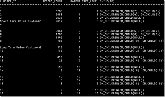
The following image shows all the clusters produced and we can see that we have the renamed cluster labels we set when we used the ODM tool.

Step 2 – Setting up the new data

There are some simple rules to consider when preparing the data for the cluster model. These really apply to all of the data mining algorithms.

- You will need to have the data prepared and in the same format as you used for building the model

- This will include the same table structure. Generally this should not be a problem. If you need to merge a number of tables to form a table with the correct format, the simplest method is to create a view.

- All the data processing for the records and each attribute needs to be completed before you run the apply function.

- Depending on the complexity of this you can either build this into the view (mentioned above), run some pl/sql procedures and create a new table with the output, etc. I would strongly suggest that the minimum pre-processing you have to do on the data the simpler the overall process and implementation will be.

- The table or view must have one attribute for the CASE_ID. The CASE_ID is an attribute that is unique for each record. If the primary key of the table is just one attribute you can use this. If not then you will need to generate a new attribute that is unique. One way to do this is to concatenate each of the attributes that form the primary key.

Step 3 – Applying the Cluster model to new data – In Batch mode

There are two ways of using an Oracle Data Mining model in the database. In this section we will look at how you can run the cluster model to score data in a batch mode. What I mean by batch mode is that you have a table of data available and you want to score the data with what the model thinks their cluster will be.

To do this we need to run the APPLY function that is part of the DBMS_DATA_MINING package.

For clustering we do not have CASE_ID, so we can leave this parameter NULL.

One of the parameters is called RESULT_TABLE_NAME. Using the DBMS_DATA_MINING.APPLY package and function, it looks to create a new table that will contain the outputs of the cluster scoring. This table (for the KMeans and O-Cluster algorithms) will contain three attributes.

CASE_ID       VARCHAR2/NUMBER
CLUSTER_ID    NUMBER
PROBABILITY   NUMBER

The table will have the CASE_ID. This is the effectively the primary key of the table.

If we take our INSURANCE_CUST_LTV table as the table containing the new data we want to score (Yes this is the same table we used to build the cluster model) and the CLUSTER_KMEANS_MODEL as the cluster model we want to use. The following codes show the APPLY function necessary to score the data.

BEGIN

DBMS_DATA_MINING.APPLY(
     model_name          => 'CLUSTER_KMEANS_MODEL',
     data_table_name     => 'INSURANCE_CUST_LTV',
     case_id_column_name => 'CUSTOMER_ID',
     result_table_name   => 'CLUSTER_APPLY_RESULT');
END;

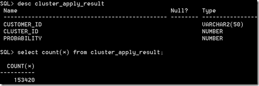
On my laptop this took 3 second to complete. This involved scoring 15,342 records, creating the table CLUSTER_APPLY_RESULT and inserting 153,420 scored records into the table CLUSTER_APPLY_RESULT.

Why did we get 10 times more records in our results table than we did in our source table ?

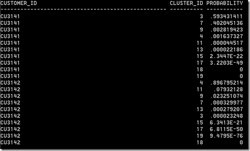
Using the batch mode i.e. using the DBMS_DATA_MINING.APPLY function it will create a record for each of the possible clusters that the record will belong too along with the probability of it belonging to that cluster. In our case we have built our clustering models based on 10 clusters.

In the following diagram we have a listing for two of the customers in our dataset, the clusters that have been assigned to them and the probability of that record/customer belonging to that cluster. We can then use this information to make various segmentation decisions based on the probabilities that each has for the various clusters.

Step 4 – Applying the Cluster model to new data – In Real-time mode

When we looked at applying a classification algorithm to new data we were able to use the PREDICTION SQL function. As clustering is an unsupervised data mining technique we will not be able to use the PREDICTION function.

Instead we have the functions CLUSTER_ID and CLUSTER_PROBABILITY.

CLUSTER_ID will tell us what cluster the record is most likely to belong too i.e. the cluster with the highest probability.

This is different to the bulk processing approach as we will only get one record/result being returned.

In the following example we are asking what cluster do these two customers most likely belong too.

SELECT customer_id,
cluster_id(cluster_kmeans_model USING *) as Cluster_Num
FROM insurance_cust_ltv
WHERE customer_id in ('CU3141', 'CU3142');

Is we look back to Step 3 above we will see that the clusters listed correspond to what we have discovered.

The next function is CLUSTER_PROBABILTY. With this function we can see what the probability of customer belonging to a particular cluster. Using the results for customer CU3141 we can see what the probability is for this cluster, along with a few other clusters.

SELECT customer_id,
       cluster_probability(cluster_kmeans_model, '3' USING *) as Cluster_3_Prob,
       cluster_probability(cluster_kmeans_model, '4' USING *) as Cluster_4_Prob,
       cluster_probability(cluster_kmeans_model, '7' USING *) as Cluster_7_Prob,
       cluster_probability(cluster_kmeans_model, '9' USING *) as Cluster_9_Prob
FROM   insurance_cust_ltv
WHERE customer_id = 'CU3141';

We can also combine the CLUSTER_ID and CLUSER_PROBABILITY functions in one SELECT statement.

In the following query we want to know what the most likely cluster is for two customers and the cluster probability.

SELECT customer_id,
       cluster_id(cluster_kmeans_model USING *) as Cluster_Num,
        cluster_probability(cluster_kmeans_model, cluster_id(cluster_kmeans_model USING *) USING *) as Cluster_Prob
FROM   insurance_cust_ltv
WHERE customer_id in ('CU3141', 'CU3142');

Check back soon for my more blog posts on performing data mining in Oracle, using the Oracle Data Miner tool (part of SQL Developer) and the in-database SQL and PL/SQL code.

I hope you have enjoyed blog posts on Oracle Data Miner and you have found them useful. Let me know if there are specific topics you would like me to cover.

Thanks

Brendan Tierney

Monday, March 11, 2013

Oracle Magazine–March/April 1999

The headline articles for the March/April 1999 edition of Oracle Magazine were on the evolving world of the DBA. With some much new technology available in the database the role of the DBA is moving from a back office type role to one having a significant strategic influence in the organisation.

Tuesday, March 5, 2013

Clustering in Oracle Data Miner–Part 4

This is a the fourth part of a five (5) part blog post on building and using Clustering in Oracle Data Miner. The following outlines the contents of each post in this series on Clustering.

The first part we looked at what clustering features exist in ODM and how to setup the data that we will be using in the examples
The second part will focus on how to building Clusters in ODM .
The third post will focus on examining the clusters produced by ODM and how to use the Clusters to apply to new data using ODM.
The fourth post will look at how you can build and evaluate a Clustering model using the ODM SQL and PL/SQL functions.
The fifth and final post will look at how you can apply your Clustering model to new data using the ODM SQL and PL/SQL functions.

With Clustering we are trying to find hidden patterns in our data. Unlike classification we a not directing the algorithms on what areas/attributes to focus on.
In my preceding post on Clustering in Oracle Data Miner I showed how you can use the Oracle Data Miner (ODM) tool, that is part of SQL Developer, to build a cluster model and to apply it to new data.
As I have shown in previous blog posts we can do all of the same steps using SQL and PL/SQL. In this blog post I will show you how to to these SQL and PL/SQL functions to generate a Clustering model and how you can evaluate the model produced.
Step 1 – What Cluster Models to we already have
Oracle Data Miner comes with a number of data dictionary tables. We can use these to see what already exists in our schema. In the example below we will have a look to see the Cluster models that were produced in the Part 2 blog post.
format model_name format a20
format mining_function format a20
format algorithm format a20
SELECT model_name,
       mining_function,
       algorithm,
       build_duration,
       model_size
FROM ALL_MINING_MODELS
WHERE mining_function = 'CLUSTERING';

We can also look at the model settings that ODM produced. We can look at the settings of the K-Means model. This model (in my case) is called CLUS_KM_1_25.
column setting_value format a20
select setting_name,
setting_value,
setting_type
from all_mining_model_settings
where model_name = 'CLUS_KM_1_25'

We can also look to see what attributes are used in the K-Mean model.
SELECT attribute_name,
       attribute_type,
       usage_type,
       target
from all_mining_model_attributes
where model_name = 'CLUS_KM_1_25'

I will show you how to use this Clustering model or the one that we are about to generate in my next blog post.
Step 2 – Creating the Setting table
When creating an Oracle Data Mining model in SQL you need to create Setting table. This will contain a record for each setting they you need to set for the algorithm you want to run. The settings table has a very basic structure and only consists of two columns. It is a good idea to create a separate Settings table for each algorithm or type of data mining you want to do. To create the settings table we run the following:
CREATE TABLE CLUSTER_SETTINGS (
Setting_Name VARCHAR2(30),
Setting_Value VARCHAR2(4000));
The next step is to define the setting we want to use. The first of these will be the actual algorithm you want to run. Oracle has two Clustering algorithms: algo_kmeans and algo_o_cluster. In the examples we are working through we are using the K-Mean algorithm and we want to set the number of clusters to 10. We are also going to set the Automatic Data Preparation (ADP) on. Here is the code.
BEGIN
   INSERT INTO CLUSTER_SETTINGS (setting_name, setting_value)
   VALUES (dbms_data_mining.algo_name, dbms_data_mining.ALGO_KMEANS);
   INSERT INTO CLUSTER_SETTINGS (setting_name, setting_value)
   VALUES (dbms_data_mining.prep_auto, dbms_data_mining.PREP_AUTO_ON);
   INSERT INTO CLUSTER_SETTINGS (setting_name, setting_value)
   VALUES (dbms_data_mining.clus_num_clusters, 10);

   COMMIT;
END;
We can check to see that these records were inserted.
column setting_value format a25
select * from CLUSTER_SETTINGS;

The other settings will be dependent on what clustering algorithm is being used. Each one has their own setting. If you do not define any additional setting Oracle will use the in-build default settings.
To see what the default settings:
column setting_value format a35
select *
from table(dbms_data_mining.get_default_settings)
where setting_name like 'KM%';

If you want to use a different value to the default, just create a new record in the CLUSTER_SETTINGS table with the new value.

Step 3 – Create the new Cluster Model
We have the algorithm settings ready, so the next steps is to create the Cluster model. We will be using the DBMS_DATA_MINING.CREATE_MODEL function and pointing it to our CLUSTER_SETTINGS table.
BEGIN
   DBMS_DATA_MINING.CREATE_MODEL(
      model_name          => 'CLUSTER_KMEANS_MODEL',
      mining_function     => dbms_data_mining.clustering,
      data_table_name     => 'INSURANCE_CUST_LTV',
      case_id_column_name => 'CUSTOMER_ID',
      target_column_name => null,
      settings_table_name => 'CLUSTER_SETTINGS');
END;
This takes a few seconds to run on my laptop. When finished we can uses queries like we used in Step 1 above to find out the details of what was produced.
Step 4 – Examining the Cluster model
The first thing that we will need to check is that the model was created.
format model_name format a20
format mining_function format a15
format algorithm format a15
SELECT model_name,
       mining_function,
       algorithm,
       build_duration,
       model_size
FROM ALL_MINING_MODELS
WHERE mining_function = 'CLUSTERING';

One thing that is a bit curious is the mode size. We have basically created two K-means models using the same settings, but the final models have different sizes. See below for an explanation.
Now lets look at the algorithms settings for our new Cluster model (Cluster KMeans Model)
select setting_name,
setting_value,
setting_type
from all_mining_model_settings
where model_name = 'CLUSTER_KMEANS_MODEL'

We can also look at the attributes used in the clusters.
SELECT attribute_name,
       attribute_type,
       usage_type,
       target
from all_mining_model_attributes
where model_name = 'CLUSTER_KMEANS_MODEL'

If we compare this list back to the list of attributes that were part of the model that we developed in the ODM tool, you will see that we have some extra attributes listed for the new K-means model.
The reason for these extra attributes and the bigger size (although still small) will be due to us having applied a sampling in the ODM tool. We took a subset of the data in the ODM tool and built the model based on this data. For the model we just created in SQL we took all the data (no sampling). That is why it would have looked at including more attributes because it was looking at a much bigger data set, etc.
Step 5 – Examining the Cluster Details
In this step we are going to look at some of the clusters produced by our new Cluster model.
We can produce the information relating to the clusters that were produced and what level in the hierarchy each cluster belongs. We can use this information to create/draw our own cluster hierarchy diagram.
set lines 90
column child format a40
select id,
       record_count,
       parent,
       tree_level,
       child
from table(dbms_data_mining.get_model_details_km('CLUSTER_KMEANS_MODEL'))

To look at the Centroid details for a particular cluster e.g. Cluster ID = 7, we can run:
column attribute_name format a25
column mode_value format a25
select t.id,
       c.attribute_name,
       c.mean,
       c.mode_value,
       c.variance
from table (dbms_data_mining.get_model_details_KM('CLUSTER_KMEANS_MODEL')) t,
     table(t.centroid) c
where t.id = 7
order by c.attribute_name
The results will contain details of the centroid for cluster number 7. The centroid details will include the attributes that were used to form the centroid and the values for each attribute.

The last thing we can look at is the rule for a cluster. The following query will give you the full details of the cluster rule for Cluster 7. This will give for each attribute what the values or ranges of values that is used for that cluster. I’ll let you run this as it returns a large number of records. Run it and have a look at some of the output.
select t.id,
       a.attribute_name,
       a.conditional_operator,
       nvl(a.attribute_str_value,
       a.attribute_num_value) AS value,
       a.attribute_support,
       a.attribute_confidence
from TABLE(dbms_data_mining.get_model_details_km('CLUSTER_KMEANS_MODEL')) t,
     TABLE(t.rule.antecedent) a
where t.id = 7
ORDER BY t.id, a.attribute_name, attribute_support, attribute_confidence desc, value;

My next blog post on Clustering in Oracle, will be the final one in the series. It will show you how to apply a Clustering model to new data in your database.

Pages