Monday, November 19, 2018

Oracle Machine Learning notebooks

In this blog post I'll have a look at Oracle Machine Learning notebooks, some of the example notebooks and then how to create a new one.

Check out my previous blog posts on ADWC.

- Create an Autonomous Data Warehouse Cloud Service

- Creating and Managing OML user on ADWC

On entering Oracle Machine Learning on your ADWC service, you will get the following.

NewImage

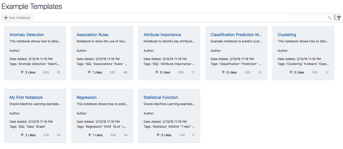
Our starting point is to example what is listed in the Examples section. Click on the Examples link. The following lists the example notebooks.

NewImage

Here we have examples that demonstrate how to build Anomaly Detection, Association Rules, Attribute Importance, Classification, Regression, Clustering and one that contains examples of various statistical function.

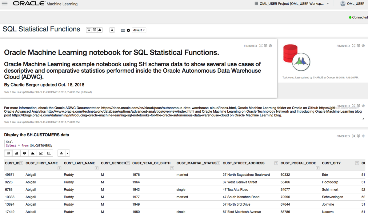
Click on one of these to see the notebook. The following is the notebook demoing the Statistical Functions. When you select a notebook it might take a few seconds to setup and open. There is some setup needed in the background and to make sure you have access to the demo data and then runs the notebook, generating the results. Most of the demo data is based on the SH schema.

NewImage

Now let us create our first notebook.

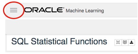
From the screen shown above lift on the menu icon on the top left of the screen.

NewImage

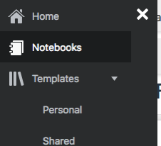
And then click on Notebooks from the pop-out menu.

NewImage

In the Notebooks screen click on the Create button to create your first notebook.

NewImage

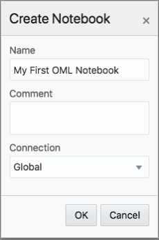
And give it a meaningful name.

NewImage

The Notebook shell will be created and then opened for you.

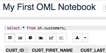
In the grey box, just under the name the name of your Notebook, is where you can enter your first SQL statement. Then over on the right hand side of this Cell you will see a triangle on its side. This is the run button.

NewImage

For now you can only run SQL statements, but you also have other notebooks features such as different charting options and these are listed under the grey cell, where your SQL is located.

NewImage

Here you can create Bar, Pie, Area, Line and Scatter charts. Here is an example of a Bar chart.

NewImage

Warning: You do need to be careful of your syntax, as minimal details are given on what is wrong with your code. Not even the error numbers.

Go give it a good and see how far you can take these OML Notebooks.

Wednesday, November 14, 2018

Reading Data from Oracle Table into Python Pandas - How long & Different arraysize

Here are some results from a little testing I recent did on extracting data from an Oracle database and what effect the arraysize makes and which method might be the quickest.

The arraysize determines how many records will be retrieved in each each batch. When a query is issued to the database, the results are returned to the calling programme in batches of a certain size. Depending on the nature of the application and the number of records being retrieved, will determine the arraysize value. The value of this can have a dramatic effect on your query and application response times. Sometimes a small value works very well but sometimes you might need a larger value.

My test involved using an Oracle Database Cloud instance, using Python and the following values for the arraysize.

arraysize = (5, 50, 500, 1000, 2000, 3000, 4000, 5000) 

The first test was to see what effect these arraysizes have on retrieving all the data from a table. The in question has 73,668 records. So not a large table. The test loops through this list of values and fetches all the data, using the fetchall function (part of cx_Oracle), and then displays the time taken to retrieve the results.

# import the Oracle Python library
import cx_Oracle
import datetime
import pandas as pd
import numpy as np

# setting display width for outputs in PyCharm
desired_width = 280
pd.set_option('display.width', desired_width)
np.set_printoptions(linewidth=desired_width)
pd.set_option('display.max_columns',30)

# define the login details
p_username = "************"
p_password = "************"
p_host = "************"
p_service = "************"
p_port = "1521"

print('--------------------------------------------------------------------------')
print(' Testing the time to extract data from an Oracle Database.')
print('    using different approaches.')
print('---')
# create the connection
con = cx_Oracle.connect(user=p_username, password=p_password, dsn=p_host+"/"+p_service+":"+p_port)

print('')
print(' Test 1: Extracting data using Cursor for different Array sizes')
print('    Array Size = 5, 50, 500, 1000, 2000, 3000, 4000, 5000')
print('')
print('   Starting test at : ', datetime.datetime.now())

beginTime = datetime.datetime.now()
cur_array_size = (5, 50, 500, 1000, 2000, 3000, 4000, 5000)
sql = 'select * from banking_marketing_data_balance_v'

for size in cur_array_size:
    startTime = datetime.datetime.now()
    cur = con.cursor()
    cur.arraysize = size
    results = cur.execute(sql).fetchall()
    print('      Time taken : array size = ', size, ' = ', datetime.datetime.now()-startTime, ' seconds,  num of records = ', len(results))
    cur.close()

print('')
print('   Test 1: Time take = ', datetime.datetime.now()-beginTime)
print('')

And here are the results from this first test.

Starting test at :  2018-11-14 15:51:15.530002
      Time taken : array size =  5  =  0:36:31.855690  seconds,  num of records =  73668
      Time taken : array size =  50  =  0:05:32.444967  seconds,  num of records =  73668
      Time taken : array size =  500  =  0:00:40.757931  seconds,  num of records =  73668
      Time taken : array size =  1000  =  0:00:14.306910  seconds,  num of records =  73668
      Time taken : array size =  2000  =  0:00:10.182356  seconds,  num of records =  73668
      Time taken : array size =  3000  =  0:00:20.894687  seconds,  num of records =  73668
      Time taken : array size =  4000  =  0:00:07.843796  seconds,  num of records =  73668
      Time taken : array size =  5000  =  0:00:06.242697  seconds,  num of records =  73668

As you can see the variation in the results.

You may get different performance results based on your location, network connectivity and proximity of the database. I was at home (Ireland) using wifi and my database was located somewhere in USA. I ran the rest a number of times and the timings varied by +/- 15%, which is a lot!

When the data is retrieved in this manner you can process the data set in the returned results set. Or what is more traditional you will want to work with the data set as a panda. The next two test look at a couple of methods of querying the data and storing the result sets in a panda.

For these two test, I'll set the arraysize = 3000. Let's see what happens.

For the second test I'll again use the fetchall() function to retrieve the data set. From that I extract the names of the columns and then create a panda combining the results data set and the column names.

startTime = datetime.datetime.now()
print('   Starting test at : ', startTime)
cur = con.cursor()
cur.arraysize = cur_array_size
results = cur.execute(sql).fetchall()
print('   Fetched ', len(results), ' in ', datetime.datetime.now()-startTime, ' seconds at ', datetime.datetime.now())
startTime2 = datetime.datetime.now()
col_names = []
for i in range(0, len(cur.description)):
    col_names.append(cur.description[i][0])
print(' Fetched data & Created the list of Column names in ', datetime.datetime.now()-startTime, ' seconds at ', datetime.datetime.now())

The results from this are.

      Fetched  73668  in  0:00:07.778850  seconds at  2018-11-14 16:35:07.840910
      Fetched data & Created the list of Column names in  0:00:07.779043  seconds at  2018-11-14 16:35:07.841093
      Finished creating Dataframe in  0:00:07.975074  seconds at  2018-11-14 16:35:08.037134

Test 2: Total Time take =  0:00:07.975614

Now that was quick. Fetching the data set in just over 7.7788 seconds. Creating the column names as fractions of a millisecond, and then the final creation of the panda took approx 0.13 seconds.

For the third these I used the pandas library function called read_sql(). This function takes two inputs. The first is the query to be processed and the second the name of the database connection.

print(' Test 3: Test timing for read_sql into a dataframe')
cur_array_size = 3000
print('   will use arraysize = ', cur_array_size)
print('')
startTime = datetime.datetime.now()
print('   Starting test at : ', startTime)

df2 = pd.read_sql(sql, con)

print('      Finished creating Dataframe in ', datetime.datetime.now()-startTime, ' seconds at ', datetime.datetime.now())
# close the connection at end of experiments
con.close()

and the results from this are.

   Test 3: Test timing for read_sql into a dataframe will use arraysize =  3000

   Starting test at :  2018-11-14 16:35:08.095189
      Finished creating Dataframe in  0:02:03.200411  seconds at  2018-11-14 16:37:11.295611

You can see that it took just over 2 minutes to create the panda data frame using the read_sql() function, compared to just under 8 seconds using the previous method.

It is important to test the various options for processing your data and find the one that works best in your environment. As with most languages there can be many ways to do the same thing. The challenge is to work out which one you should use.

Tuesday, November 6, 2018

Installing and configuring Oracle 18c XE

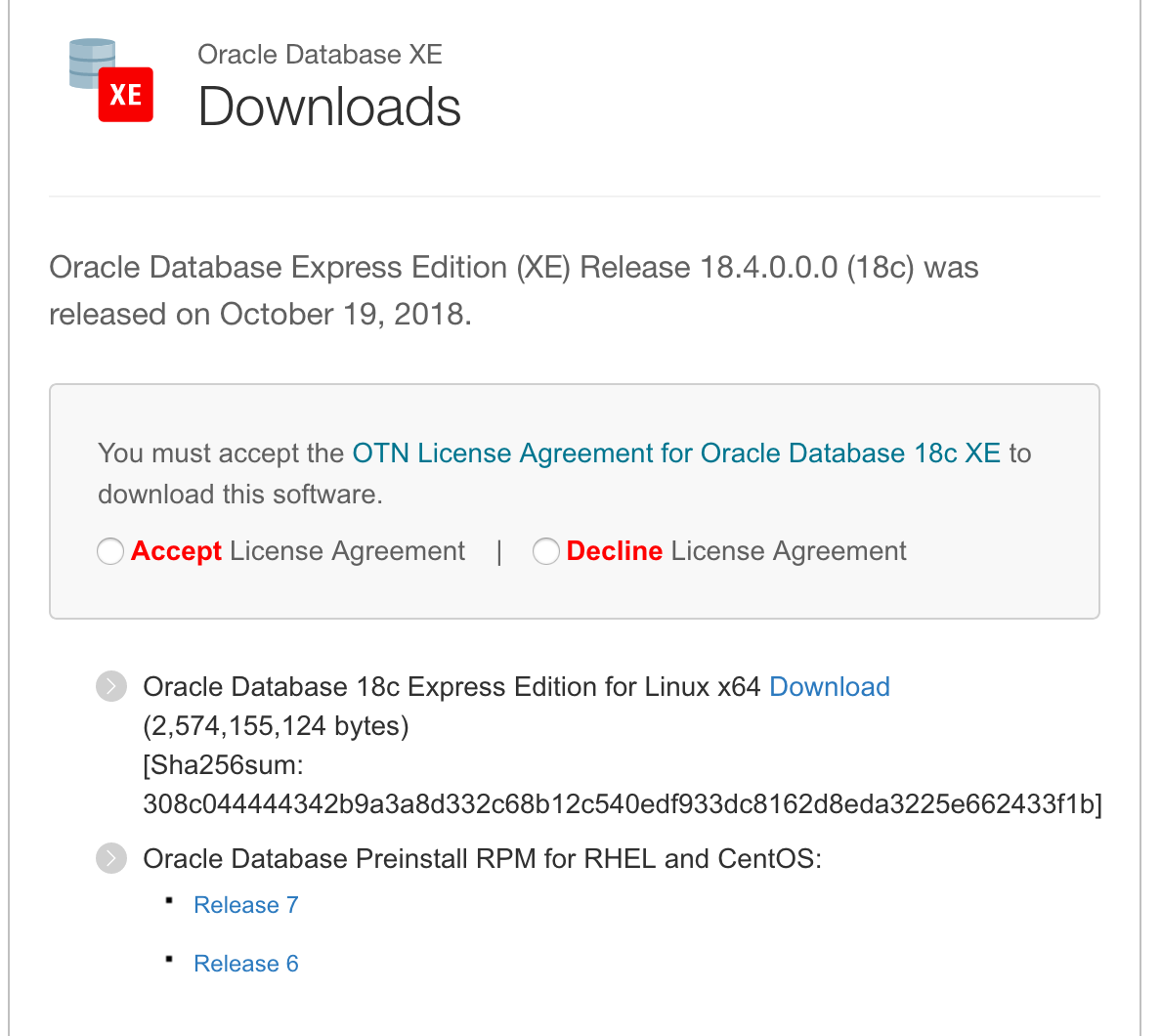
The following are the simple steps required to install Oracle 18c XE (express edition) on Oracle Linux. Check out my previous blog post on Oracle 18c XE. Also check out the product webpage for more details and updates. There is a very important word on that webpage. That word is 'FREE' and is something you don't see too often. Go get and use the (all most) full enterprise version of the Oracle Database.

I've created a VM using Oracle Linux for the OS.

After setting up the VM, login as root and download the RPM file.

NewImage

Run the following as root to perform dependency checks and configurations.

yum install -y oracle-database-preinstall-18c 

You can now run the install using the following command.

yum -y localinstall oracle-database-xe-18c-1.0-1.x86_64.rpm. 

When the install has completed, the next step is to install the database. This is done using the following command.

/etc/init.d/oracle-xe-18c configure 

You will be prompted to enter a common password for the SYS, SYSTEM and PDBADMIN users. You will need to change these at a later time.

Then to start the database, run

systemctl start oracle-xe-18c 

The next time you restart the VM, you might find that the database hasn't started or loaded. You will need to do this manually. This is a bit of a pain in the behind.

To avoid having to do this each time, run the following commands as root.

systemctl daemon-reload
systemctl enable oracle-xe-18c

These commands will allow the database to be shutdown when the machine or VM is being shutdown and will automatically start up the database when the machine/VM startups again.

The final step is to connect to the database

sqlplus sys///localhost:1521/XE as sysdba 

You can then go and perform all your typical admin tasks, set up SQLDeveloper, and create additional users.

Bingo! All it good now.

Docker

Putting Oracle 18c XE on docker is an excellent way to make it easily deployable and to build out solutions that require a DB.

Check out these links for instructions on how to setup a Docker container with Oracle 18c XE.

https://github.com/fuzziebrain/docker-oracle-xe

Sunday, October 28, 2018

RandomForests in R, Python and SQL

I recently wrote a two part article explaining how Random Forests work and how to use them in R, Python and SQL.

These were posted on ToadWorld webpages. Check them out.

Part 1 of article


Part 2 of article

Tuesday, October 23, 2018

Creating and Managing OML users on Oracle ADWS

(Check out my recent blog post on getting the ADWS up and running. You will need to have following those before you can perform the following steps.

In this post I'll look at how to setup and manage users specifically for the Oracle Machine Learning (OML) tool. This tool is only available on ADWS and is a zeppelin based notebook for analytics, data science and machine learning.

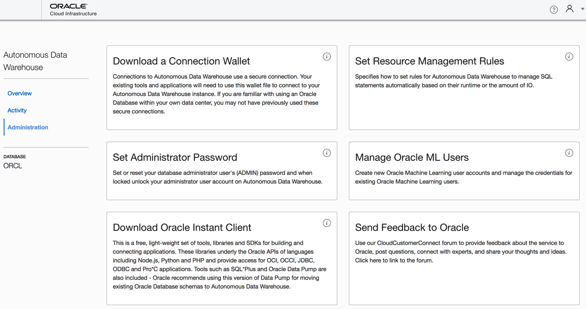
1. Open the service console for ADWS and click on Administration Administration can be found on the small menu list on the left hand side of the screen. NewImage

2. Click on Manage Oracle ML Users As we are only interested in OML and Users for OML, just click on the section titled 'Oracle ML Users'

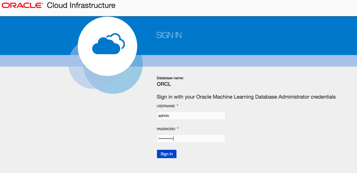
3. Sign-in as Admin user This user was created in my previous blog post. Hopefully you can remember the password. NewImage

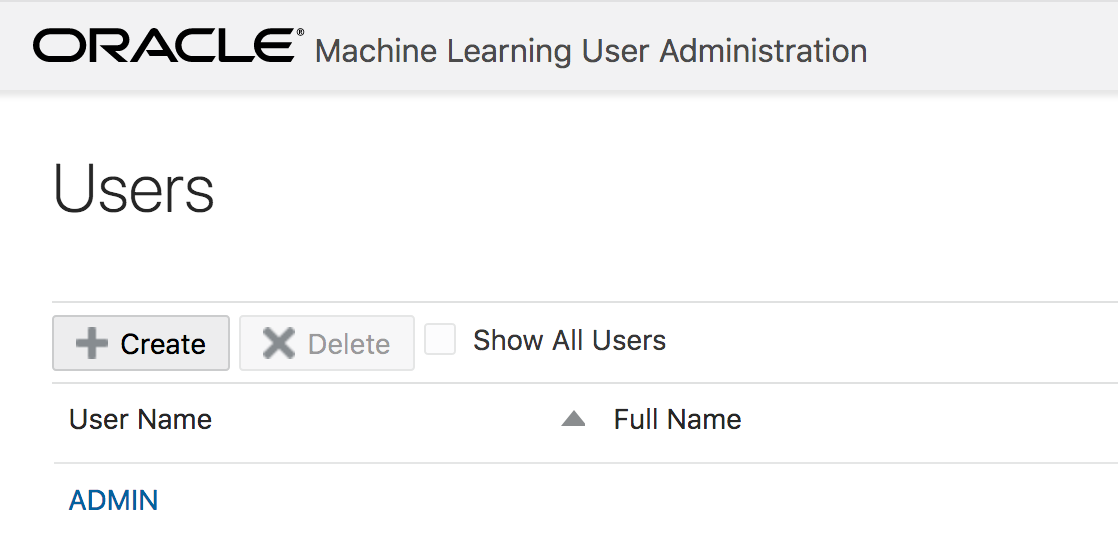
4. Create a New User The only user currently enabled for OML is the Admin user. To create a new OML user click on the Create button

NewImage

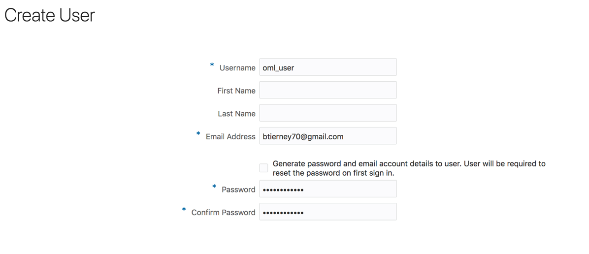
5. Enter OML User details Enter the details of the OML user. Enter an email address and the person will receive an email with their login details. You have the choice of having a system generated password or uncheck the tick box and add in a password. NewImage Click the Create button. And hopefully the user will receive the email. The email may take a little bit of time to arrange in the users email box!

6. Log into Oracle Machine Learning

You have 2 options. The first is to follow the link in the email or click on the Home button on the top right hand side of the screen. NewImage

You will then be logged into Oracle Machine Learning. Look out for my blog posts on using this product and how to run the demos. NewImage

Slides from my OOW Presentation

Here are the slides from my presentation (with Neil Chandler) at Oracle Open World and Oracle Code One.

1 - Code1-Nnets_REST-joint-ver2 NewImage

Saturday, October 20, 2018

Oracle 18c XE - Comes with in-database and R machine learning

As of today 20th October, Oracle has finally released Oracle 18c XE aka Express Edition

A very important word associated with Oracle 18c XE is the word 'FREE'

Yes it is FREE

This FREE product is backed full of features. Think of all the features that come with the Enterprise Edition of the Database. It comes with most of those features, including some of the extra add on features.

I said it comes with most features. There are a few features that don't come with XE, so go check out the full list here.

NewImage

There are a few restrictions:

  • Up to 12 GB of user data
  • Up to 2 GB of database RAM
  • Up to 2 CPU threads
  • Up to 3 Pluggable Databases

I know of so many companies and applications that easily meet the above restrictions.

For the Data Scientists and Machine Learning people, the Advanced Analytics option is now available with Oracle 18c XE. That means you can use the in-memory features for super fast analytics, use the in-database machine learning algorithms, and also use the embedded R feature called Oracle R Enterprise.

Yes you are limited to 12G of user data. That might be OK for most people but for those whose data is BIG then this isn't an option for you.

There is a phrase, "Your data isn't as big as you think", so maybe your data might fit within the 12G.

Either way this can be a great tool to allow you to try out machine learning for Free in a test lab environment.

Go download load it and give it a try.

Thursday, October 18, 2018

Creating an Autonomous Data Warehouse Cloud Service

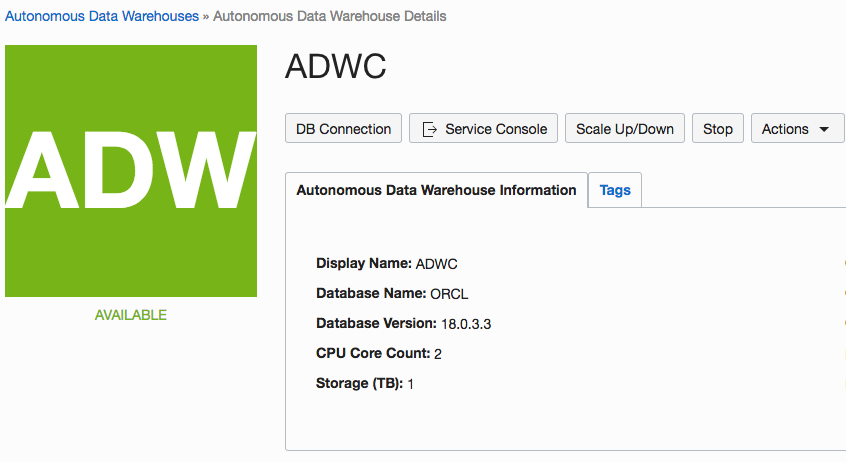
The following outlines the steps to create a Autonomous Data Warehouse Cloud Service.
Log into your Oracle Cloud account and then follow these steps.
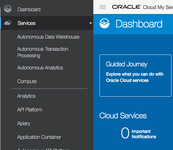
1. Select Autonomous Data Warehouse Cloud service from the side menu
NewImage
2. Select Create Autonomous Data Warehouse button
NewImage
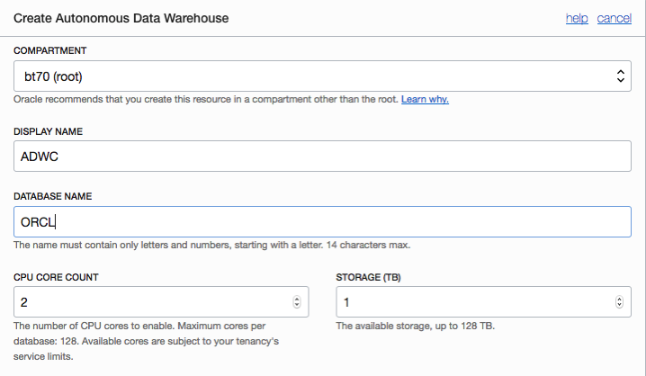
3. Enter the Compartment details (Display Name, Database Name, CPU Core Count & Storage)
NewImage
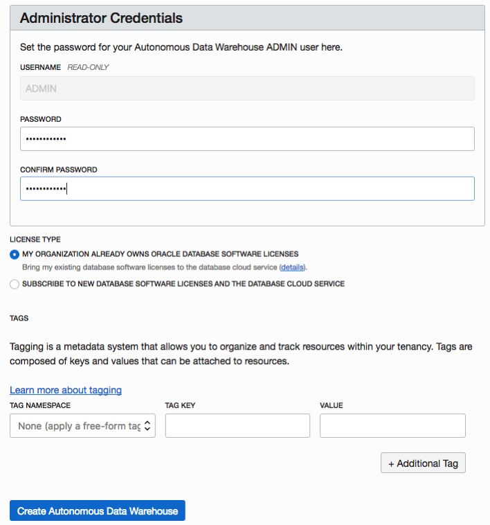
4. Enter a Password for Administrator, and then click ‘Create Autonomous Data Warehouse’
NewImage
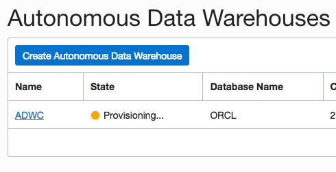
5. Wait until the ADWC is provisioned
Going from this
NewImage
to this
NewImage
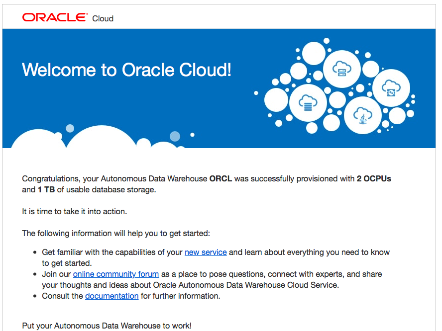
And you should receive and email that looks like this
NewImage
6. Click on the name of the ADWS you created
NewImage
7. Click on the Service Console button
NewImage
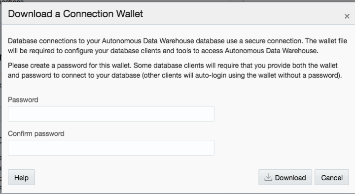
8. Then click on Administration and then Download a Connection Wallet
Specify the password
NewImage
You an now use this to connect to the ADWS using SQL Developer
All done.

Monday, October 15, 2018

R vs Python vs SQL for Machine Learning (Infographic)

Next week I'll be giving several presentation on machine learning at Oracle Open World and Oracle Code One. In one of these presentation an evaluation of using R vs Python vs SQL will be given and discussed.

Check out the infographic containing the comparisons.

Click here to download the PDF version.

Info Graphic

Wednesday, October 10, 2018

OOW 2018 Chocolate Tasting

Calling all Oracle ACEs, Developer Champions and Oracle Product Managers from around the World.

Are you going to Oracle Open World or Oracle Code One?

If you are, bring some of your favourite chocolates from where you live and share them with other Oracle ACEs, Developer Champions and Oracle PMs.

Location : The Hub (Moscone West).

Date : Wednesday 24th October

Time : 3pm-4pm

All you have to do is to bring some of the best chocolate from your country or your favourite chocolate, meet with other people, talk about Oracle technologies and what you have learned during your time at Oracle Open World and Oracle Code One.

Please don't bring your typical high street, mass market type of chocolate. Bring the good stuff. Pick it up at your local chocolate shop or in the airport as you begin your travels.

Last year (2017) we had chocolate from 14 different countries. They were all very different and very tasty.

I'll have some Butlers Chocolates with me for the tasting. What chocolates will you bring?

Friday, September 7, 2018

OOW18 and Code One agendas with Date and Times

I've just received an email in from the organisers of Oracle Open World (18) and Oracle Code One (formally Java One) with details of when I will be presenting.

It's going to be a busy presenting schedule this year with 4 sessions.

It's going to be a busy presenting schedule this year with 3 sessions on the Monday.

Check out my sessions, dates and times.

Screenshot 2018 09 07 09 10 11

In addition to these sessions I'll also be helping out in the Demo area in the Developer Lounge. I'll be there on Wednesday afternoon handing out FREE beer.

Wednesday, August 29, 2018

Bringing Neural Networks to Production using GraphPipe

Machine learning is a fascinating topic. It has so much potential yet very few people talk about using machine learning in production. I've been highlighting the need for this for over 20 years now and only a very small number of machine learning languages and solutions are suitable for production use. Why? maybe it is due to the commercial aspects and as many of the languages and tools are driven by the open source community, one of the last things they get round to focusing on is production deployment. Rightly they are focused at developing more and more machine learning algorithms and features for developing models, but where the real value comes is will being able to embed machine learning model scoring in production system. Maybe this why the dominant players with machine learning in enterprises are still the big old analytics companies.

Yes that was a bit a of a rant but it is true. But over the summer and past few months there has been a number of articles about production deployment.

But this is not a new topic. For example, we have Predictive Model Markup Language (PMML) around for a long time. The aim of this was to allow the interchange of models between different languages. This would mean that the data scientist could develop their models using one language and then transfer or translate the model into another language that offers the same machine learning algorithms.

But the problem with this approach is that you may end up with different results being generated by the model in the development or lab environment versus the model being used in production. Why does this happen? Well the algorithms are developed by different people/companies and everyone has their preferences for how these algorithms are implemented.

To over come this some companies would rewrite their machine learning algorithms and models to ensure that development/lab results matched the results in production. But there is a very large cost associated with this development and ongoing maintenance as the models evolved. This would occur, maybe, every 3, 6, 9, 12 months. Somethings the time to write or rewrite each new version of the model would be longer than its lifespan.

These kind of problems have been very common and has impacted on model deployment in production.

In the era of cloud we are now seeing some machine learning cloud solutions making machine learning models available using REST services. These can, very easily, allow for machine learning models to be included in production applications. You are going to hear more about this topic over the coming year.

But, despite all the claims and wonders and benefits of cloud solutions, it isn't for everyone. Maybe at some time in the future but it mightn't be for some months or years to come.

So, how can we easily add machine learning model scoring/labeling to our production systems? Well we need some sort of middleware solutions.

Given the current enthusiasm for neural networks, and the need for GPUs, means that these cannot (easily) be deployed into production applications.

There have been some frameworks put forward for how to enable this. Once such framework is called Graphpipe. This has recently been made open source by Oracle.

Graphpipe

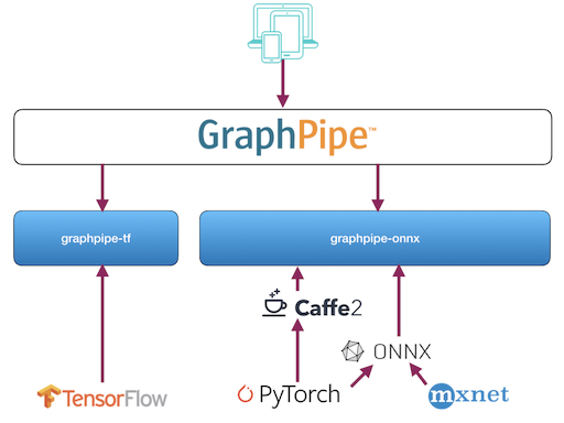
Graphpipe is a framework that to access and use machine learning models developed and running on different platforms. The framework allows you to perform model scoring across multiple neural networks models and create ensemble solutions based on these. Graphpipe development has been focused on performance (most other frameworks don't). It uses flatbuffers for efficient transfer of data and currently has integration with TensorFlow, PyTorch, MXNet, CNTK and via ONNX and caffe2.

Expect to have more extensions added to the framework.

Graphpipe website

Graphpipe getting started

Graphpipe blogpost

Graphpipe download