Friday, January 25, 2019

How long does it take to build a Machine Learning model using Oracle Cloud

Everyday someone talks about the the processing power needed for Machine Learning, and the vast computing needed for these tasks. It has become evident that most of these people have never created a machine learning model. Never. But like to make up stuff and try to make themselves look like an expert, or as I and others like to call them a "fake expert".

When you question these "fake experts" about this topic, they huff and puff about lots of things and never answer the question or try to claim it is so difficult, you simply don't understand.

Having worked in the area of machine learning for a very very long time, I've never really had performance issues with creating models. Yes most of the time I've been able to use my laptop. Yes my laptop to build models large models. In a couple of these my laptop couldn't cope and I moved onto a server.

But over the past few years we keep hearing about using cloud services for machine learning. If you are doing machine learning you need to computing capabilities that are available with cloud services.
So, the results below show the results of building machine learning models, using different algorithms, with different sizes of data sets.

For this test, I used a basic cloud service. Well maybe it isn't basic, but for others they will consider it very basic with very little compute involved.

I used an Oracle Cloud DBaaS for this experiment. I selected an Oracle 18c Extreme edition cloud service. This comes with the in-database machine learning option. This comes with 1 OCPUs, 7.5G Memory and 170GB storage. This is the basic configuration.


Next I created data sets with different sizes. These were based on one particular data set, as this ensures that as the data set size increases, the same kind of data and processing required remained consistent, instead of using completely different data sets.

The data set consisted of the following number of records, 72K, 660K, 210K, 2M, 10M and 50M.
I then created machine learning models using Decisions Tree, Naive Bayes, Support Vector Machine, Generaliszd Linear Models (GLM) and Neural Networks. Yes it was a typical classification problem.
The following table below shows the length of time in seconds to build the models. All data preparations etc was done prior to this.

Note: It should be noted that Automatic Data Preparation was turned on for these algorithms. This performed additional algorithm specific data preparation for each model. That means the times given in the following tables is for some data preparation time and for building the models.


Converting the above table into minutes.


It is clear that the Neural Network model takes a lot longer to build than all the other algorithms. In this test the Neural Network model had only one hidden layer.

When we chart the build timings, leaving out Neural Networks, we get.
 
We can see Naive Bayes, Decision Tree, GLM and SVM algorithms have very similar model build timings, but as the data volumes increase the Decision Tree algorithm become less efficient.

Overall it doesn't take a long time to build models. In a way it is a very trivial task!

I mentioned at the start of this post I had created a data set of 50M records. Unfortunately I wasn't able to get models build for this data set using this cloud instance. It used used so much TEMP tablespace that the file volumes on my cloud instance ran out of space!

I suppose if I wanted to go bigger with my data, I needed a bigger boat!
I haven't included any timings for model scoring using these models. Why? the scored data is immediately returned event for large the largest data sets.
 

Monday, January 14, 2019

Changing the markers for Google Maps and centering map

In some recent work, I've been integrating with Google Maps and some of the other Google API's a lot. This post is just a reminder for myself on how to change the format, colour, and other properties of the map pointers.

cluster_0_gmap = gmaps.symbol_layer(
    map_locations_c0, fill_color='red',
    stroke_color='red', scale=5 )

cluster_1_gmap = gmaps.symbol_layer(
    map_locations_c1, fill_color='green',
    stroke_color='green', scale=5 )

cluster_2_gmap = gmaps.symbol_layer(
    map_locations_c2, fill_color='purple',
    stroke_color='purple', scale=5 )

cluster_3_gmap = gmaps.symbol_layer(
    map_locations_c3, fill_color='blue',
    stroke_color='blue', scale=5 )

And now for the map initial settings, centred on Athlone town in the middle of Ireland.

fig = gmaps.figure()

figure_layout = {
'width': '950px',
'height': '730px',
'border': '1px solid black',
'padding': '1px',
'margin': '0 auto 0 auto'
}

ireland_coord = (53.42, -7.94)
fig=gmaps.figure(center=ireland_coord, zoom_level=7.5, layout=figure_layout)

fig.add_layer(cluster_0_gmap)
fig.add_layer(cluster_1_gmap)
fig.add_layer(cluster_2_gmap)
fig.add_layer(cluster_3_gmap)
fig

Friday, January 4, 2019

Understanding, Building and Using Neural Network Models using Oracle 18c

I recently had an article published on Oracle Developer Community website about Understanding, Building and Using Neural Network Machine Learning Models with Oracle 18c. I've also had a 2 Minute Tech Tip (2MTT) video about this topic and article.

NewImage

Oracle 18c Database brings prominent new machine learning algorithms, including Neural Networks and Random Forests. While many articles are available on machine learning, most of them concentrate on how to build a model. Very few talk about how to use these new algorithms in your applications to score or label new data. This article will explain how Neural Networks work, how to build a Neural Network in Oracle Database, and how to use the model to score or label new data. What are Neural Networks?

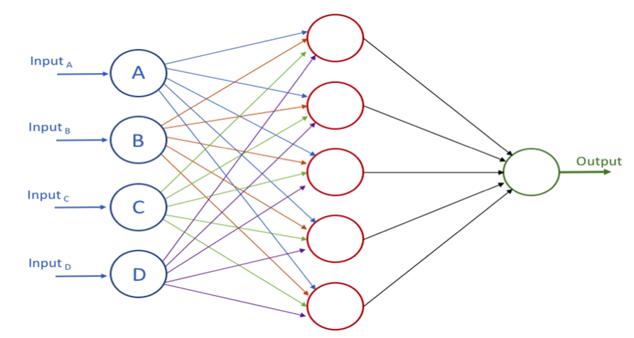
Over the past couple of years, Neural Networks have attracted a lot of attention thanks to their ability to efficiently find patterns in data—traditional transactional data, as well as images, sound, streaming data, etc. But for some implementations, Neural Networks can require a lot of additional computing resources due to the complexity of the many hidden layers within the network. Figure 1 gives a very simple representation of a Neural Network with one hidden layer. All the inputs are connected to a neuron in the hidden layer (red circles). A neuron takes a set of numeric values as input and maps them to a single output value. (A neuron is a simple multi-input linear regression function, where the output is passed through an activation function.) Two common activation functions are logistic and tanh functions. There are many others, including logistic sigmoid function, arctan function, bipolar sigmoid function, etc.

Continue reading the rest of the article here.

NewImage